StarRocks Query Optimizer

This post is a summary of the CMU Seminar on March 31, 2025, the topic of which is StarRocks Query Optimizer.

• CMU Seminar Video：StarRocks Query Optimizer (Kaisen Kang)

• CMU Seminar PDF：StarRocks Query Optimizer (Kaisen Kang)

• Chinese version of this post: StarRocks 查询优化器

StarRocks Query Optimizer Overview

Development History of StarRocks

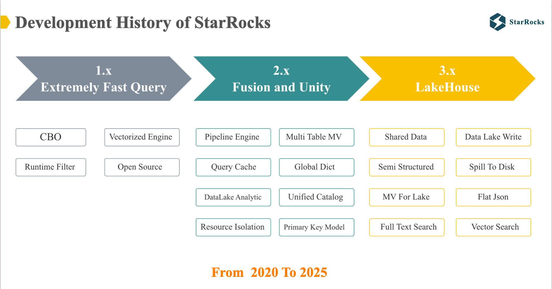
To begin, allow me to provide a concise overview of the StarRocks development journey. Over the past five years, we’ve launched three major versions:

• StarRocks version 1: built an extremely fast OLAP database, leveraging a vectorized execution engine and Cost-Based Optimizer
• StarRocks version 2: Evolved into a high-performance, unified OLAP database, introducing features like the primary key model, data lake analytics, and comprehensive query optimizations.
• StarRocks version 3: built an Open LakeHouse architecture, driven by storage and compute separation, materialized views, and advanced data lake analytics.

StarRocks Architecture

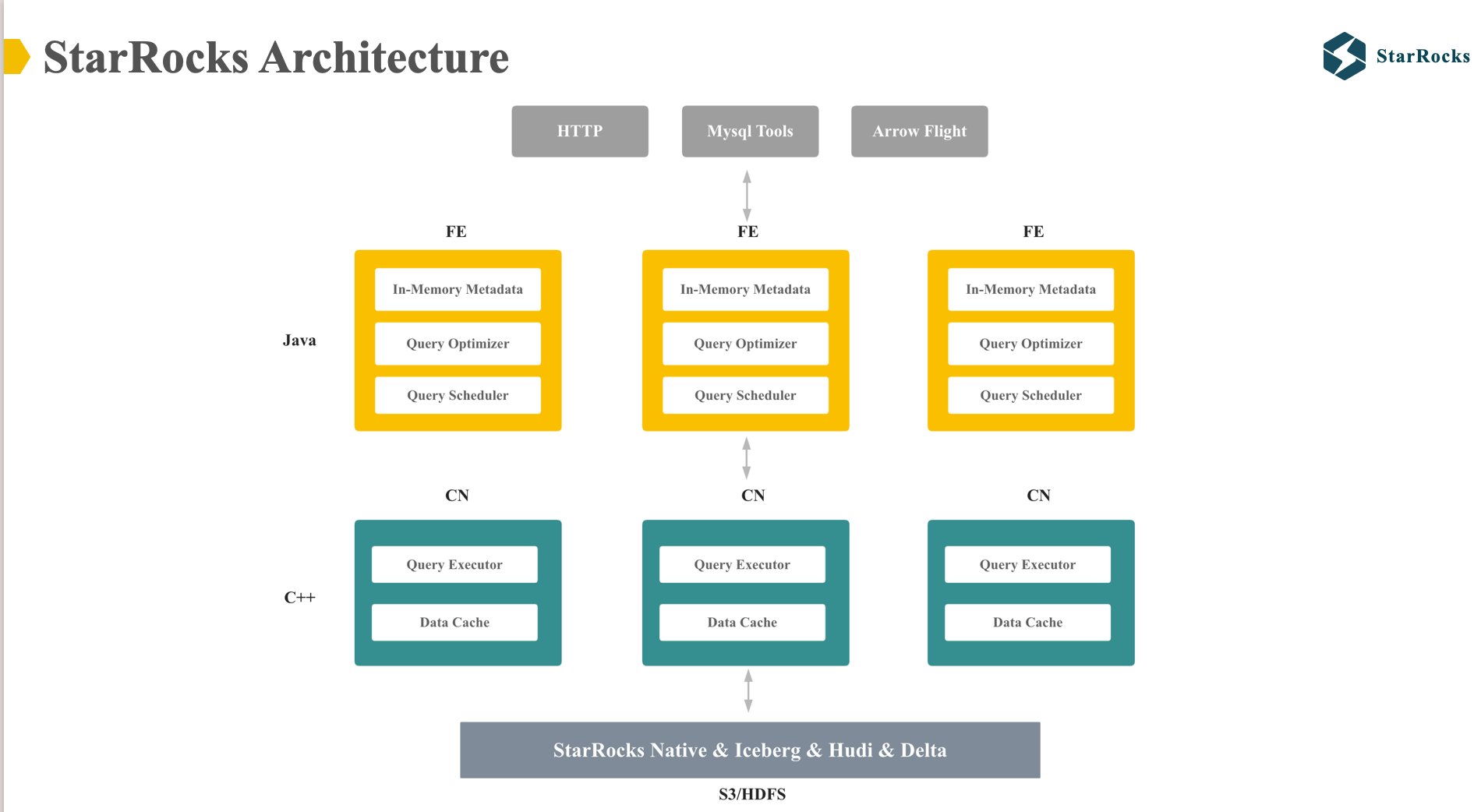
This diagram illustrates the overall architecture of StarRocks, which includes two components: Frontend and Compute Node.

• Frontend is responsible for managing in-memory metadata, query optimization, and query scheduling. It is implemented in Java.
• Compute Node handle data cache from the data lake and query execution. It is implemented in C++.

StarRocks Optimizer OverView

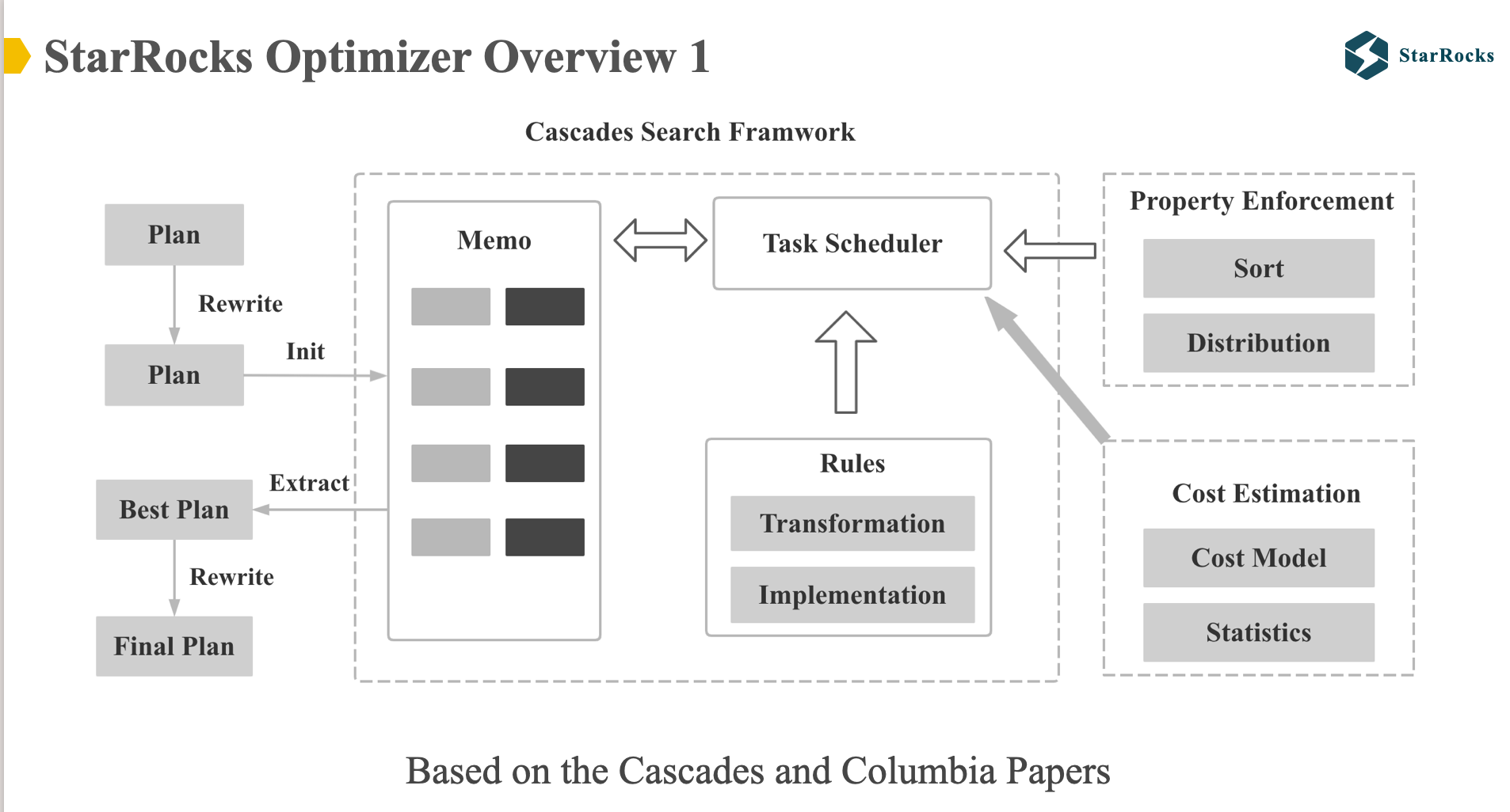
The diagram shows the overall architecture of the StarRocks optimizer. The overall framework of the StarRocks optimizer is implemented based on the Cascades and Columbia papers. The memo data structure, search framework, rule framework, and property enforce of the StarRocks optimizer are consistent with the Cascades.

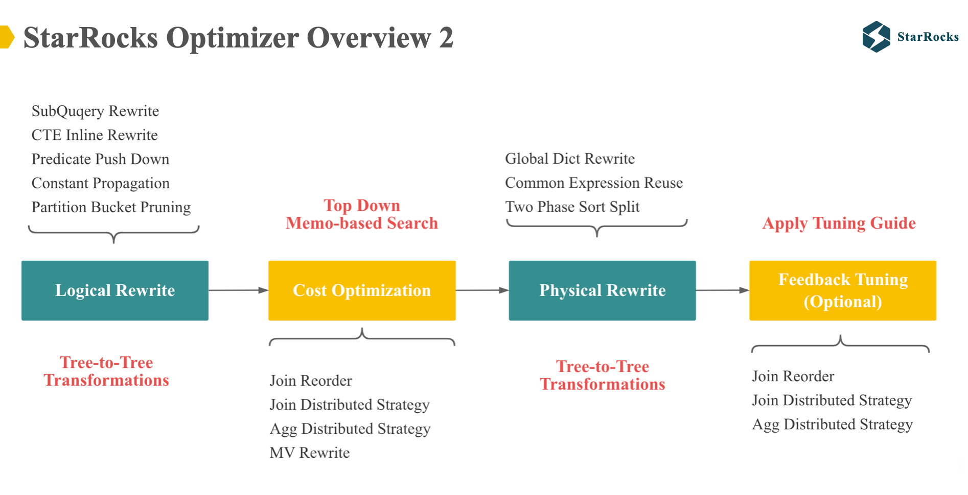
The diagram shows a more detailed optimization process of the StarRocks optimizer, and also reflects several differences with the Cascades framework.

• StarRocks optimizer uses a multi-phase optimization strategy, including Logical Rewrite, Cost-Based Optimization, Physical Rewrite, and Feedback Tuning.

• Specifically, the Logical Rewrite phase performs tree-to-tree transformations, applying a suite of common rewrite rules, such as subquery Rewrite and Common Table Expression inlining

• The Cost-Based Optimization phase leverages the Cascades Memo structure and includes important cost-based rules, including join reorder, join distribution strategy selection, aggregate distribution strategy selection, and materialized view rewrite.

• The output of the Cost-Based Optimization phase is a distributed physical tree. Subsequently, the Physical Rewrite phase executes a few physical rewrites that do not affect the cost, including Global Dictionary Rewrite, which will be discussed in detail today, and common expression reuse

• The last feedback tuning is a new feature implemented in 2024, which will be shared later. Feedback tuning adjusts the execution plan based on the feedback information at runtime.

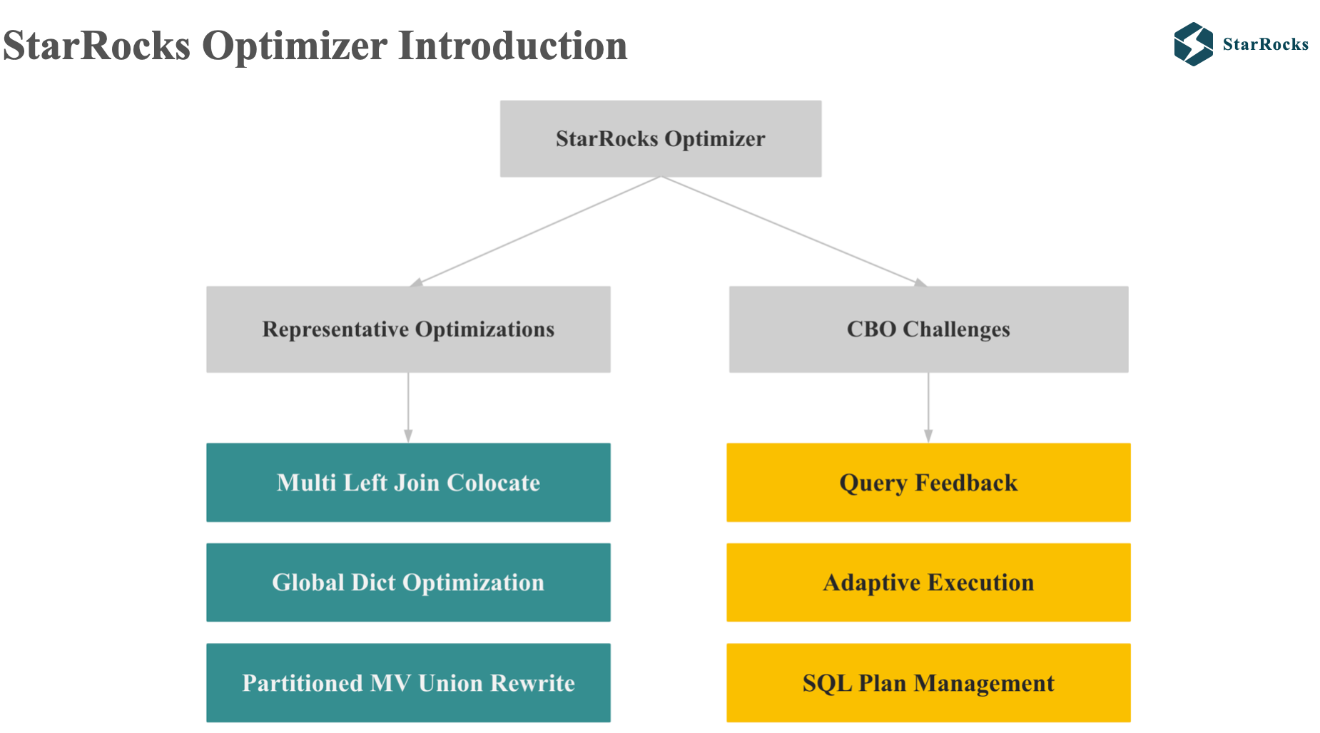
Now that we have a general understanding of StarRocks optimizer, let’s take a deeper look at it. I’ll focus on two key areas:

three representative optimizations, and second, StarRocks’ approaches to addressing common cost estimation challenges.

• The three representatives optimizations we’ll explore are: Multi-Left Join Colocate, Global Dictionary Optimization, and Partitioned Materialized View Union Rewrite.

• The three solutions to cost estimation problems include: Query Feedback, Adaptive execution, SQL plan management

Three Representative Optimizations

Multi Left Join Colocate

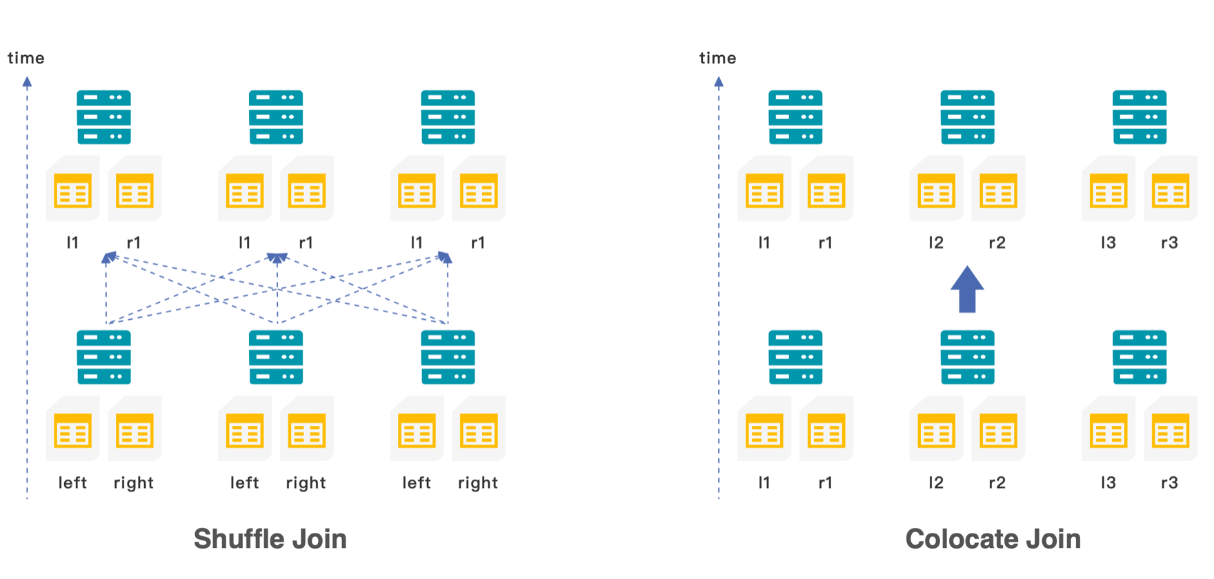
In distributed databases, the distributed execution strategies of join include: shuffle join, broadcast join, replication join, colocate join.

• Shuffle Join involves redistributing the data of both tables to the same execution node based on the join key, which needs network data transmission

• Colocate Join, in contrast, leverages pre-distributed data where both tables are already co-located on the same node according to the join key, enabling local join execution without network data transmission.

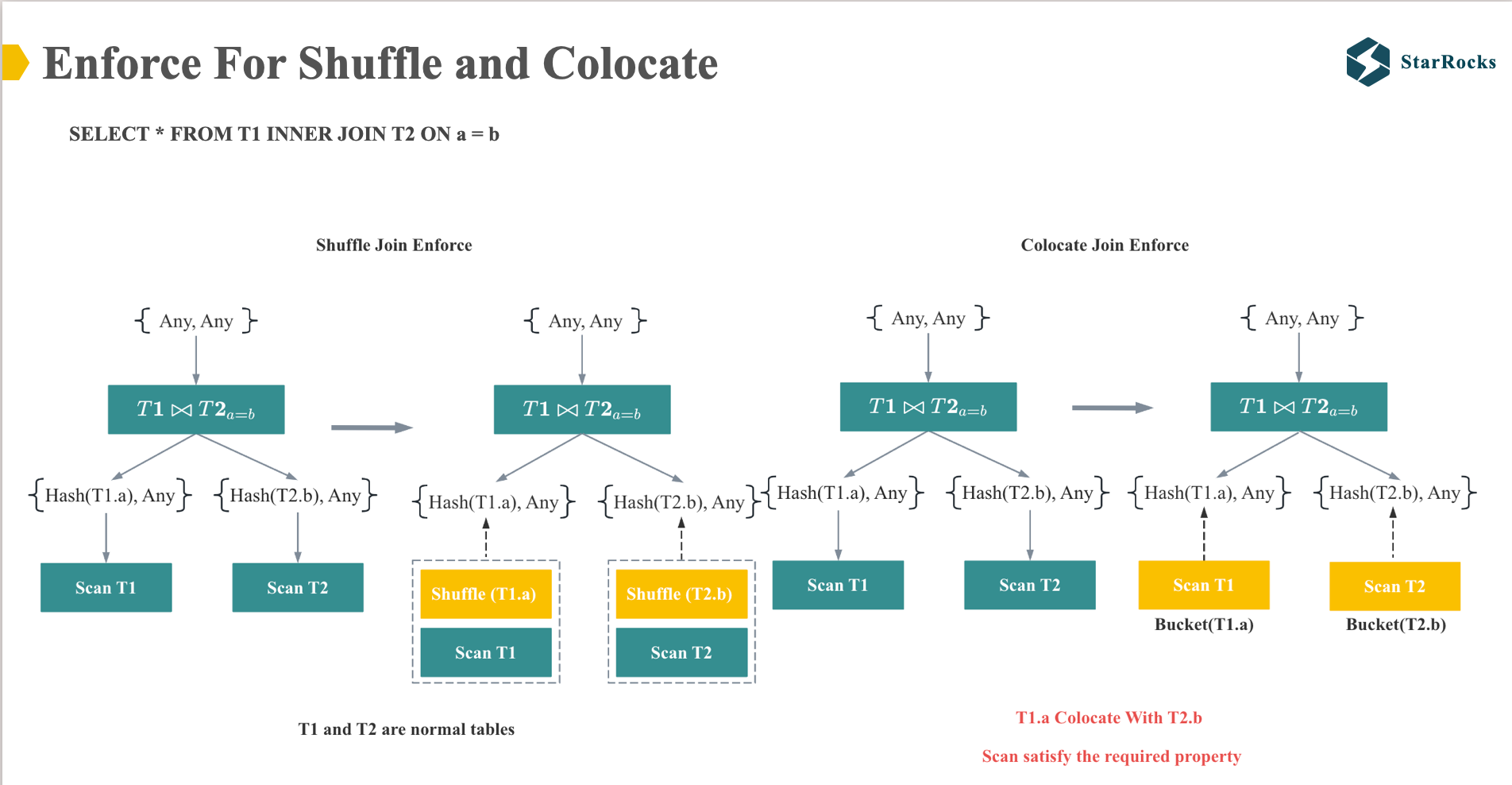
In StarRocks, the distribution strategy for join operations is determined by the distribution property enforcer.

On the left, we see an example of a Shuffle Join enforcer. The Join operator requires the distribution properties hash(T1.a) and hash(T2.b). Since T1 and T2 are normal tables that do not inherently satisfy these distribution requirements, Shuffle Exchange operators are enforced on the Scan T1 and Scan T2 operators.

On the right, we have an example of a Colocate Join enforcer. The Join operator still requires the distribution properties hash(T1.a) and hash(T2.b). However, in this case, T1 and T2 are collocated tables, pre-distributed according to the hash of T1.a and T2.b. Consequently, the required distribution properties are already satisfied, eliminating the need for Shuffle Exchange operators and enabling direct local join execution.

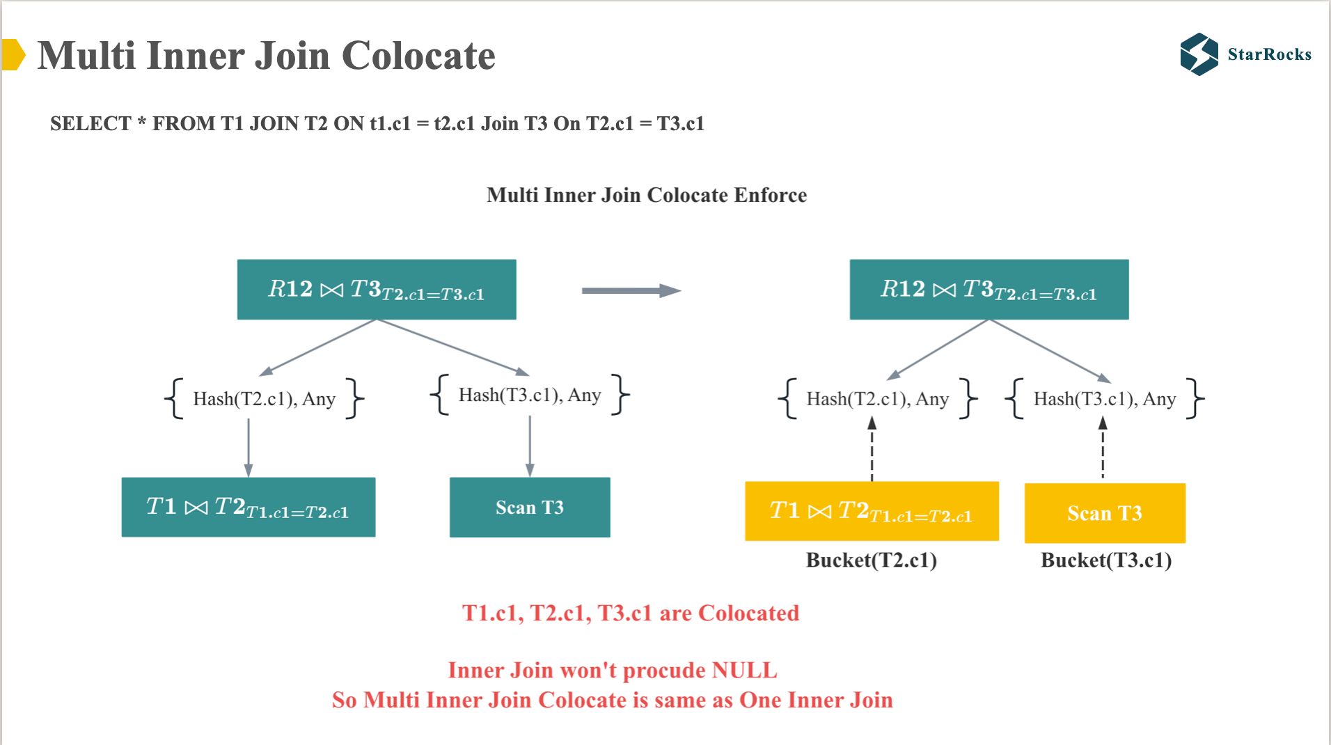
Now, let’s examine Multi-Inner Join Colocation. As illustrated in the diagram, after T1, T2, and T3 are co-located based on their respective bucket columns, the colocation process for both two-table and multi-table joins becomes identical, enabling direct local join execution. This is because after the inner join of T1 and T2, the physical distribution of inner join result is exactly the same as T1 or T2.

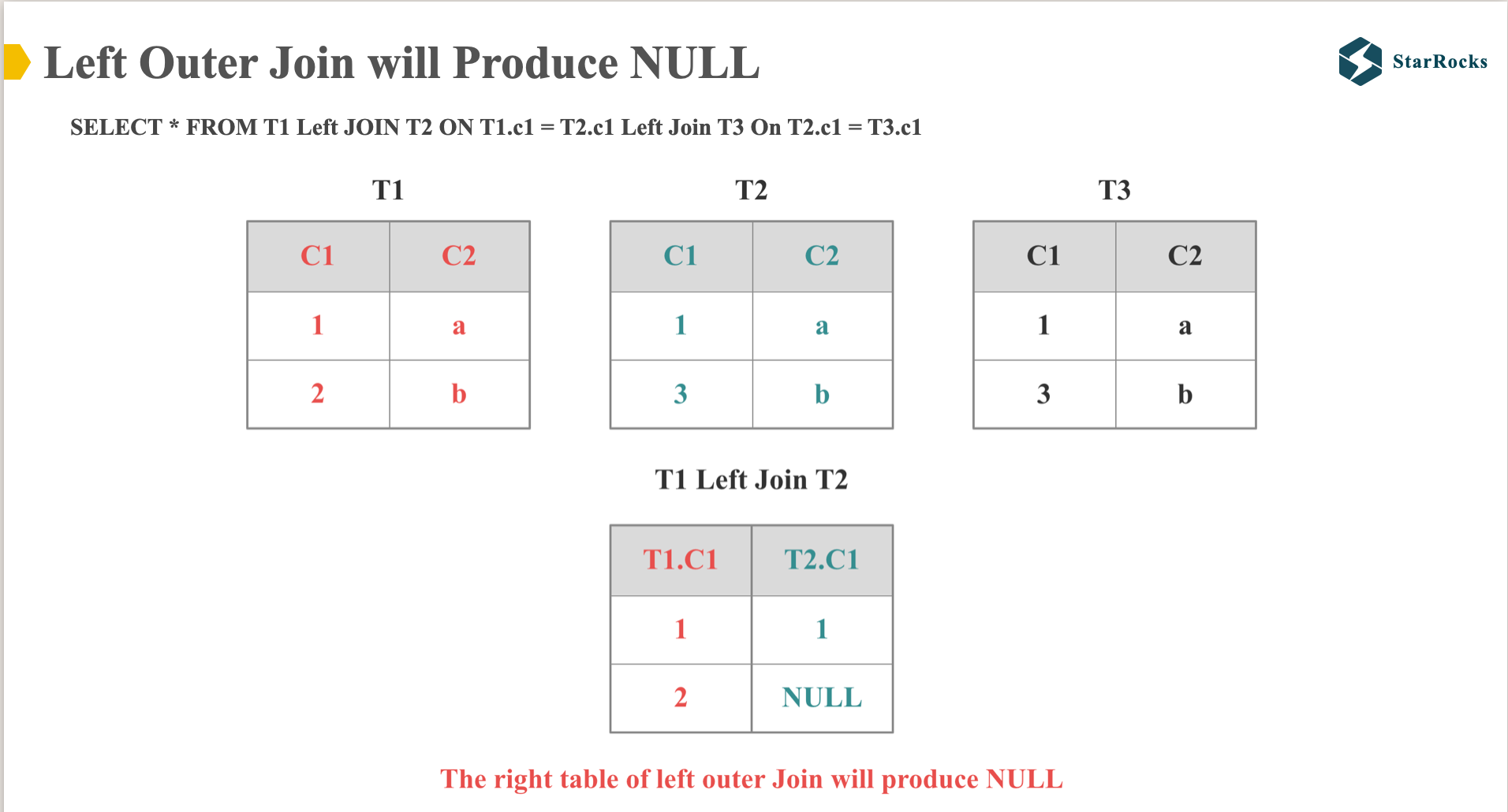
Before introducing Multi Left Join Colocate, let’s first confirm the core difference between left join and inner join:

We all know that Left Join preserves all rows from the left table, and for any rows in the left table that lack a corresponding match in the right table, the corresponding columns in the right table are populated with NULL values. As shown in the diagram, the second row in column C1 of table T2 is assigned a NULL value

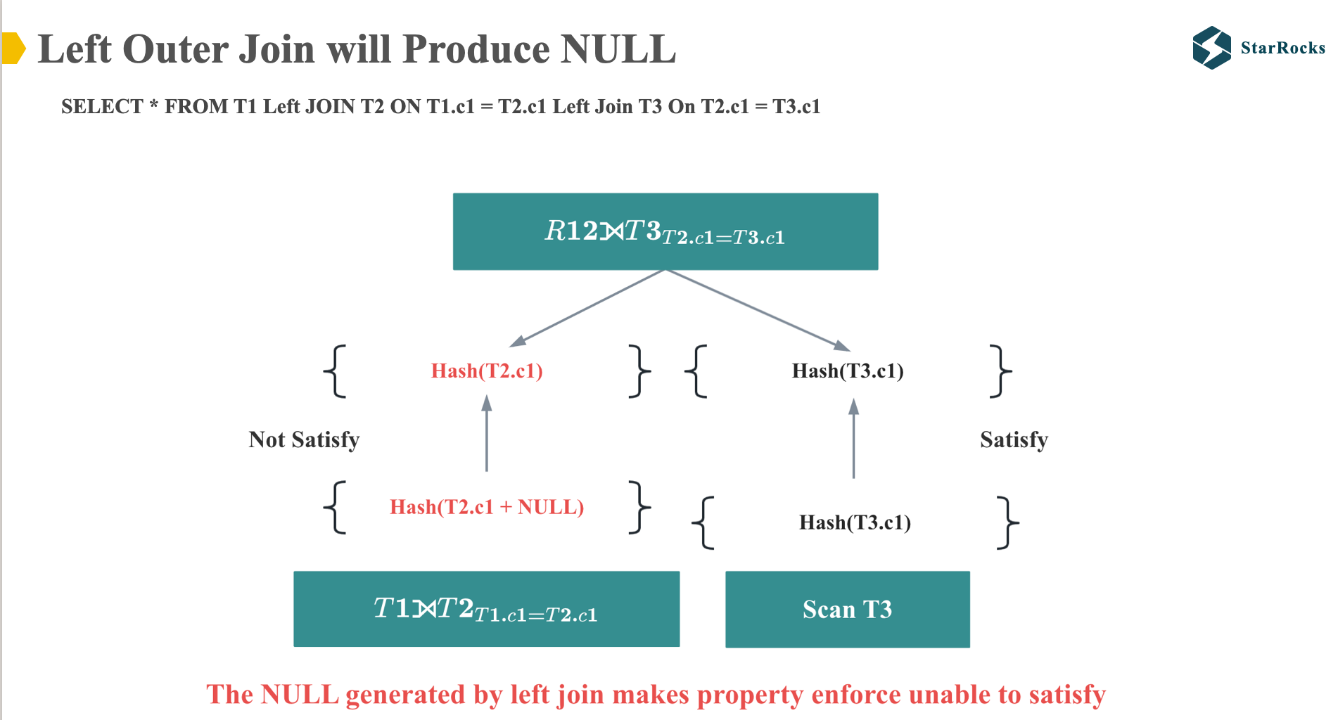
Consequently, when the multi-table Left Join distribution property enforcer is applied, the C1 column of T2 table after the Left Join operation differs from the C1 column of the original T2 table, the required distribution properties unable to satisfy, which prevents the execution of a Colocation Join.

However, let’s analyze it further to see if this left join SQL really cannot do colocate join.

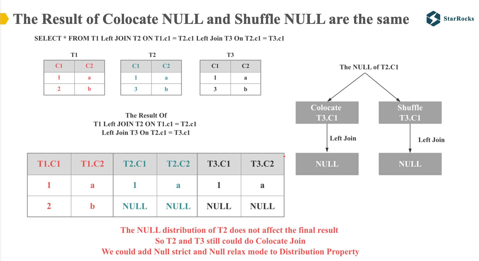
First, observe the table on the left, which shows the real results of the Left Join SQL.

Next, examine the diagram on the right and consider whether the NULL values in T2.C1 would yield differing results between Colocate Join and Shuffle Join. We understand that a NULL value compared to any value will always evaluate to NULL. Consequently, regardless of how the NULL values in T2.C1 and their corresponding T3.C1 values are distributed, whether they reside on the same execution node or not, the join result remains NULL

Therefore, we can infer that the distribution of NULL values does not impact the feasibility of a Colocation Join between T2 and T3.

Given that the non-null values in T2 and T3 satisfy the Colocation distribution requirements, T2 and T3 can indeed be Colocation Joined.

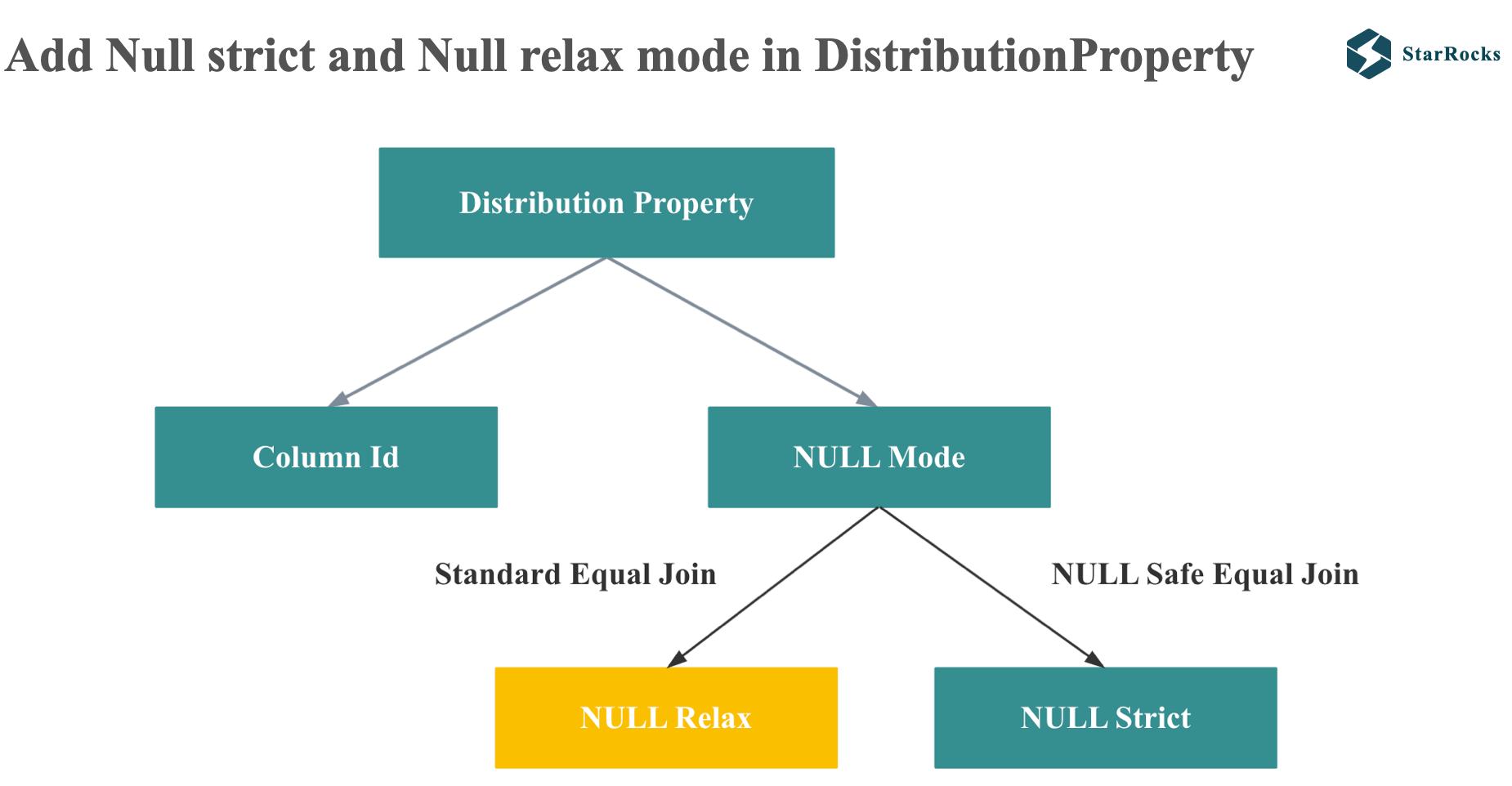
So, in order to make the distribution property enforcer support this case, StarRocks introduces NULL relax and null strict mode in the distribution property.

For the null rejecting join on predicate, StarRocks will generate NULL relax mode and ignore NULL values when comparing properties.

Conversely, for NULL-safe equal joins, StarRocks generates a NULL-strict mode, ensuring that NULL values are considered when comparing properties.

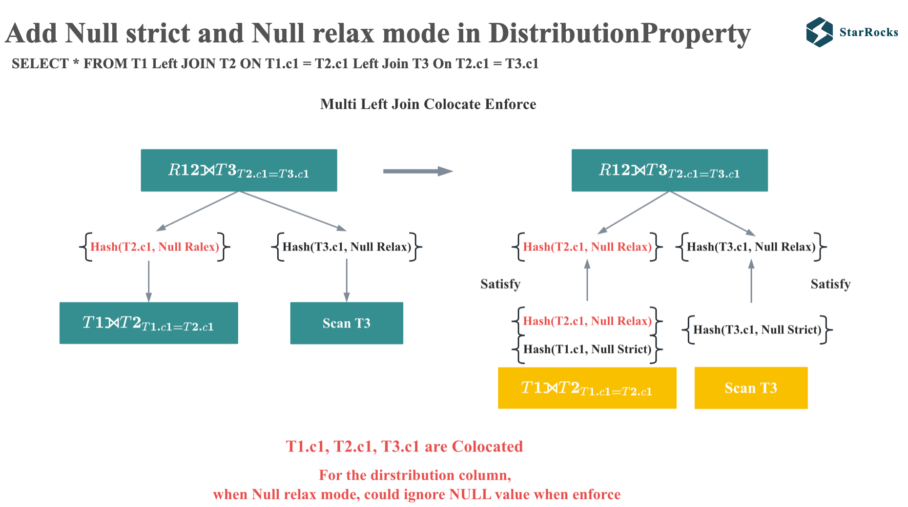
With the implementation of NULL-relax and NULL-strict modes, we can now examine the multi-table Left Join enforcement process.

Since the parent require the hash t2.c1 with null-relax mode, and the child also produce the hash t2.c1 with null-relax mode, so it satisfies the distribution property requirements of the parent node during enforcement, thereby enabling Colocation Join.

Low Cardinality Global Dict Optimization

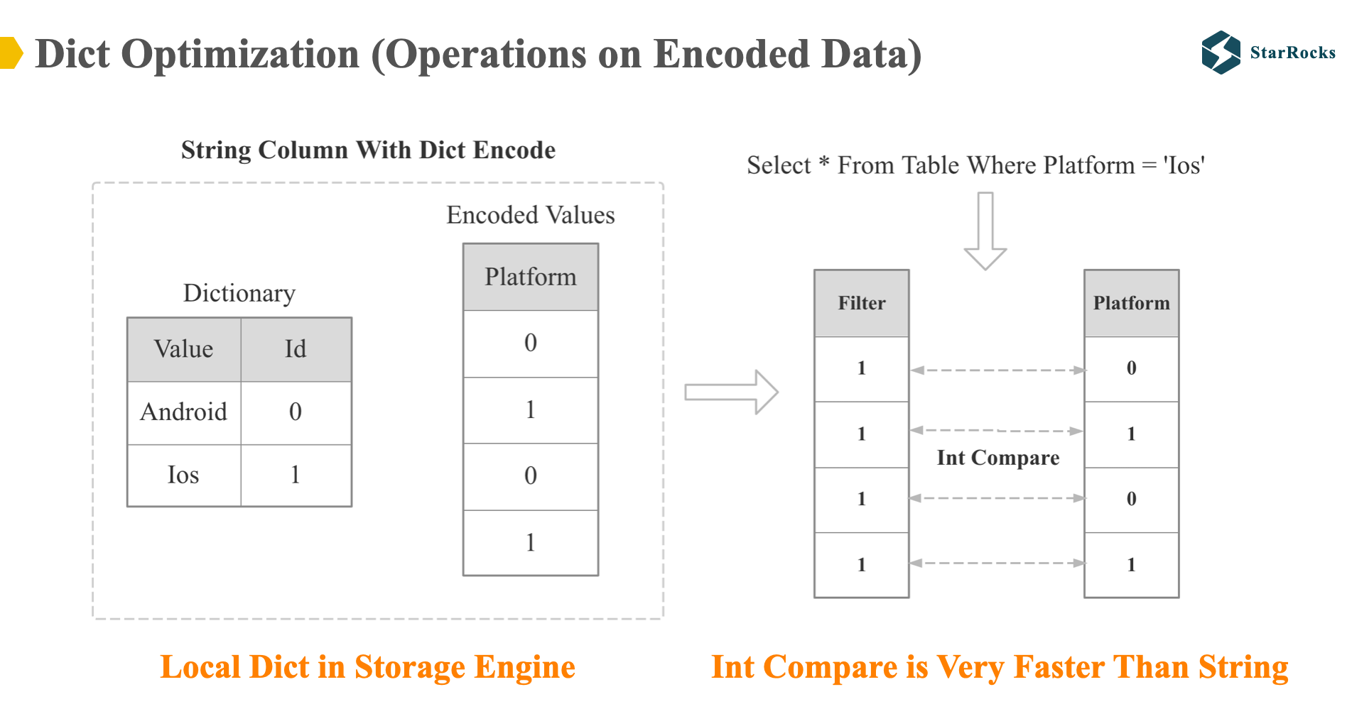
To begin, let’s define dictionary optimization. Dictionary optimization is Operations on Encoded Data. For dictionary-encoded data, computations are performed directly based on the encoded data without decoding first.

As illustrated in the diagram, the platform column is dictionary-encoded at the storage layer, so the filtering operation of platform will be directly based on the encoded integer data, the platform equal ‘IOS’ will become ‘one’ equal zero or ‘one’ equal one. int comparison will be much faster than string comparison.

Dict Optimization at the storage layer is supported by StarRocks 1.0, but only supports filter operations, and the optimization scenarios are very limited. So in StarRocks 2.0, we support global low-cardinality dictionary optimization.

A key word here is low cardinality, because if cardinality is high, the cost of maintaining the global dictionary in a distributed system will be very high. Therefore, our current cardinality limit is relatively low, and the default configuration is 256. For many dimension table string columns, 256 is enough.

Importantly, StarRocks’ global dictionary implementation is entirely transparent to users. Users do not need to care about which columns, when and how to build the global dictionary

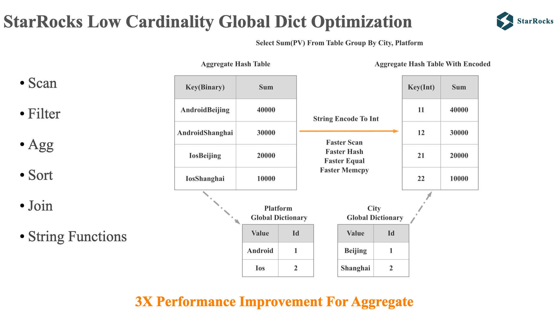
Leveraging the global dictionary, our dictionary optimization extends support to a broader range of operators and functions, including Scan, Aggregation, Join, and various commonly utilized string functions. The diagram illustrates an example of global dictionary optimization applied to a GROUP BY operation. StarRocks maintains a global dictionary for the ‘city’ and ‘platform’ columns. During the GROUP BY operation, StarRocks transforms the string-based GROUP BY into an integer-based GROUP BY, resulting in significant performance gains for operations such as Scan, Hashing, equal, and memory copying. This optimization typically yields an overall query performance improvement of three times.

Given that today’s session focuses on optimizer, let’s focus on how StarRocks uses the global dictionary to rewrite the plan.

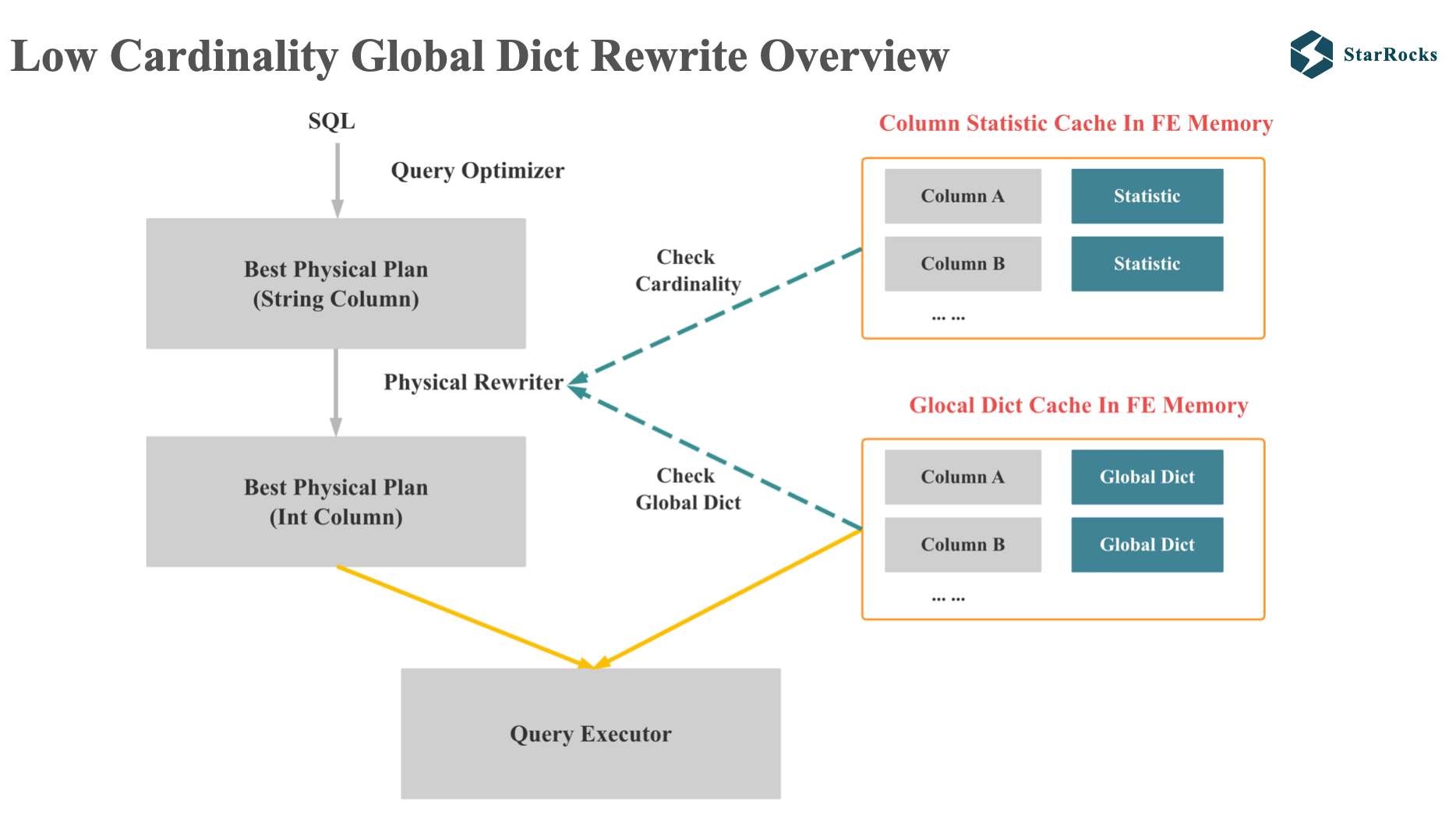
This diagram provides a high-level schematic representation of the global dictionary plan rewriting process.

Firstly, the rewriting operation takes place during the Physical Rewrite phase. We transform low-cardinality string columns into integer columns.

For successful rewriting, two conditions must be satisfied:

• the string column in the plan is a low cardinality column
• The FE memory has a global dictionary corresponding to the string column

Upon successful rewriting, the global dictionary along with the modified execution plan, are transmitted to the query executor.

This diagram provides a detailed representation of the global dictionary plan rewriting process. Currently, StarRocks supports optimization for string and array-of-string data types.

The entire rewriting process operates on the physical execution tree, employing a bottom-up traversal approach. If a string column could do low-cardinality optimization, it is rewritten as an integer column, and all string and aggregate functions referencing this column are modified accordingly. Conversely, if low-cardinality optimization couldn’t be done at a particular operator, a decode operator is inserted. At this decode operator, the integer column is transformed back into a string column.

Partitioned MV Union Rewrite

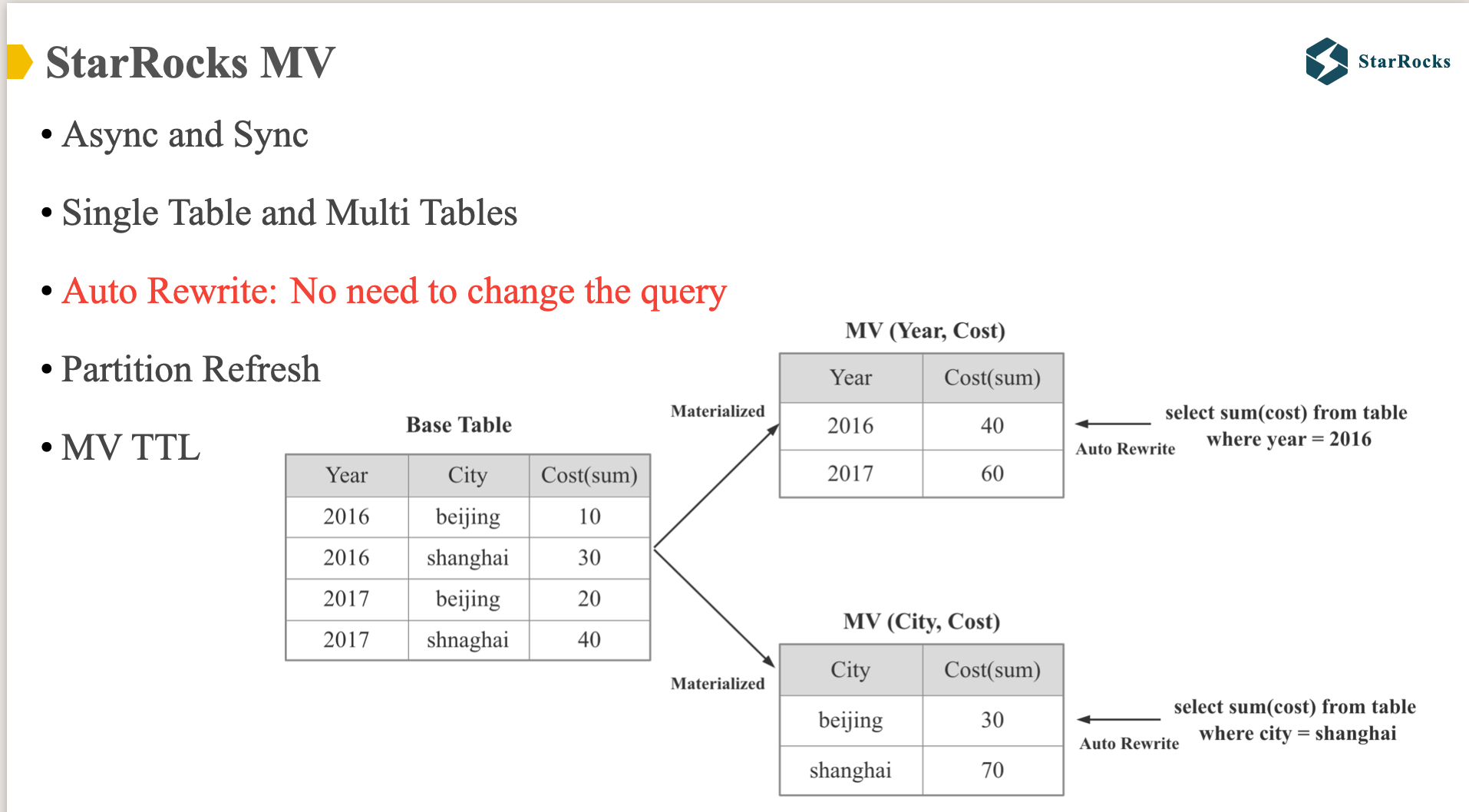
StarRocks has provided support for synchronous Materialized Views since version 1.0, and elevated MVs to a core feature in version 2.0. We have introduced support for new asynchronous MVs, expanded from single-table MV capabilities to multi-table MV support, and implemented significant optimization enhancements in automatic MV query rewriting. Today’s presentation will focus on the MV query rewriting aspect

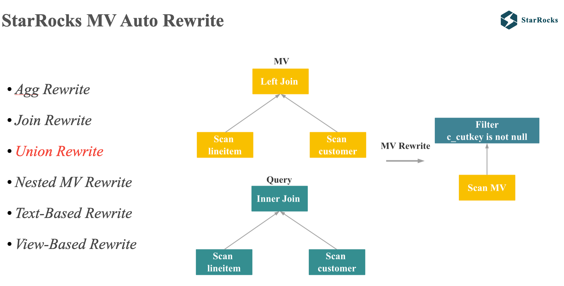
StarRocks currently supports automatic Materialized View rewriting across a wide range of scenarios, including aggregation rewrite, join rewrite, UNION rewrite, nested MV rewrite, text-based rewrite for complex SQL queries, and view-based rewrite for the sql with view.

Today, I will focus on UNION rewrite.

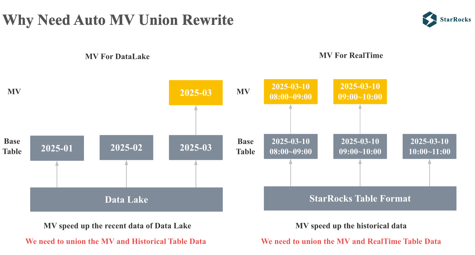
First, let’s think about why we need Auto MV Union Rewrite

The first case is the query on data lake scenario. StarRocks can directly query data lake table formats. If you expect to achieve sub-second performance, you can use MV to speed up queries on the data lake, but most users only focus on query performance in the recent period, so they only need to build MV for the data in the last week or the last month. However, users may occasionally query data in the last two weeks or the last two months. At this time, the optimizer needs to automatically rewrite the query and union the recent MV data with the historical data lake data.

The second case is a real-time scenario. We expect to use MV to achieve millisecond-level queries and tens of thousands of QPS, but the refresh of MV has a delay and cannot guarantee that the latest data is consistent with the base table. To ensure users receive accurate and up-to-date query results, we need to union the MV data with the latest data in the base table.

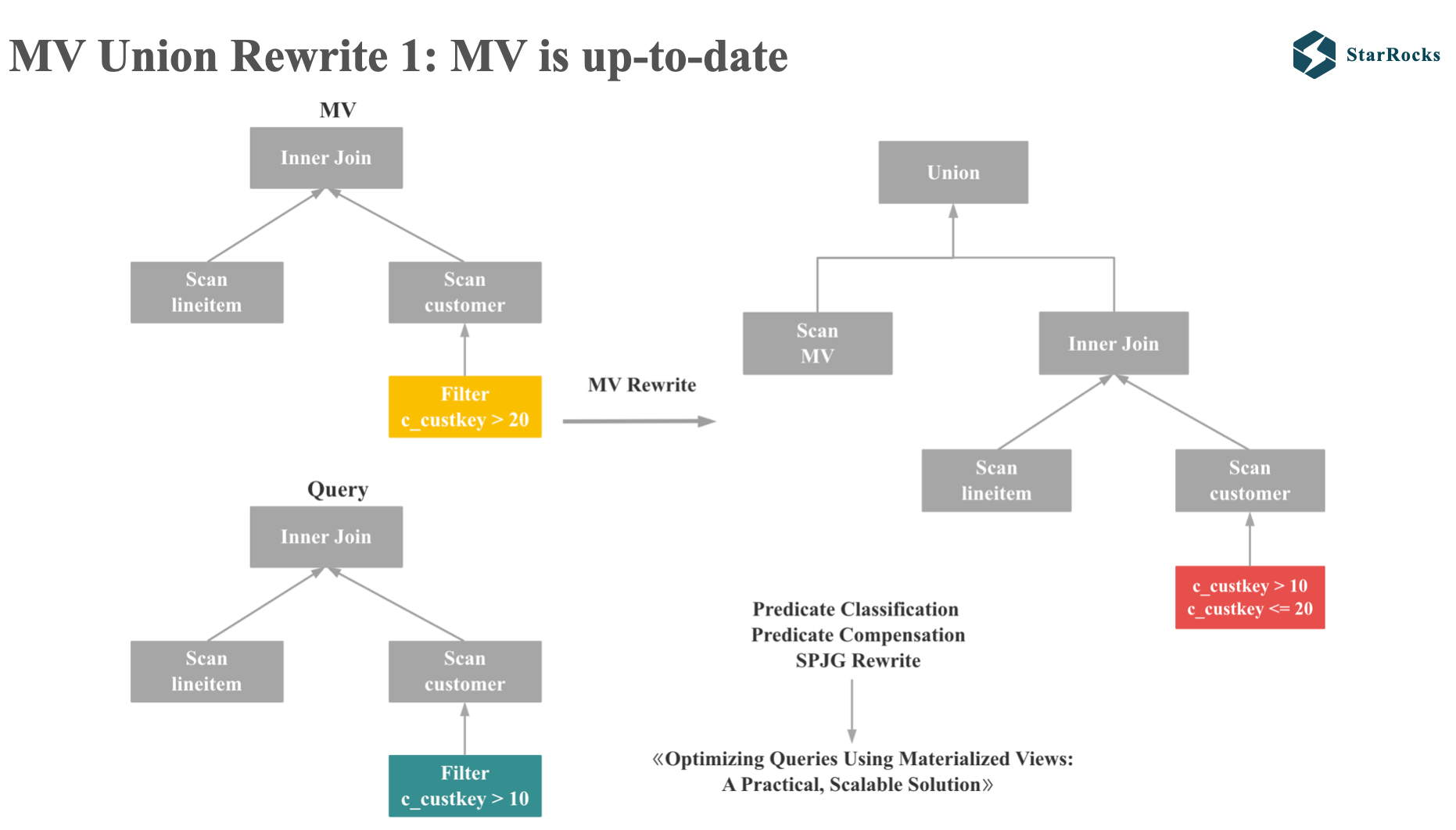
Let’s first consider the case where all partitions of the MV are refreshed:

As illustrated in the diagram, the query and Materialized View both involve simple inner joins, but with differing predicate ranges. Since the MV result set is a subset of the query result set, we must generate a compensation predicate to append to the original query, and subsequently perform a UNION operation. In this example, the compensation predicates are custkey > 10 and custkey < 20.

The predicate classification and compensation logic implemented in StarRocks aligns with the approach described in Microsoft’s research paper, <<Optimizing Queries Using Materialized Views: A Practical, Scalable Solution>>

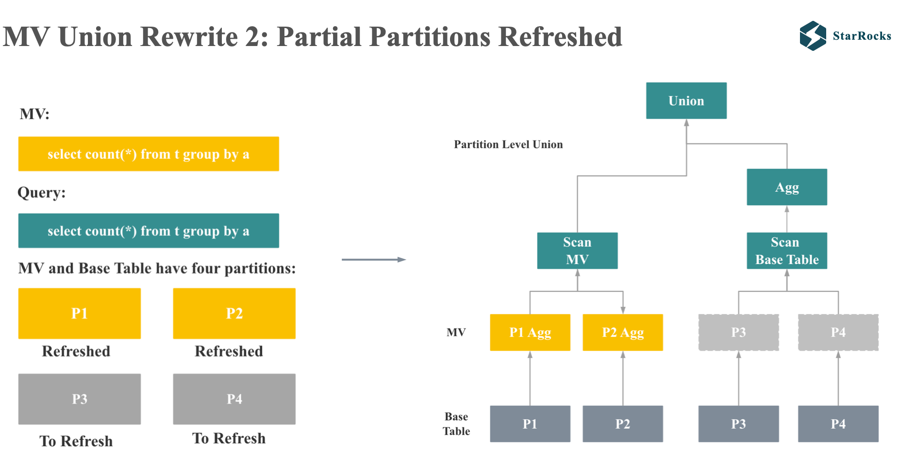
Next, let’s consider the case of Partial MV Partitions Refreshed:

If both MV and query are simple group by count queries, MV and base table both have 4 partitions, of which P1 and P2 partitions of MV have been refreshed, but P3 and P4 have not been refreshed. The rewrite of this aggregate query will become the union of the MV query and the query of the original table.

The left child of the union is the scan node of the MV, and the right child of the union is the plan of the original query. The only difference for the original query is that the partition of Scan becomes the partition of MV that has not been refreshed. in this example, which are P3 and P4 partition.

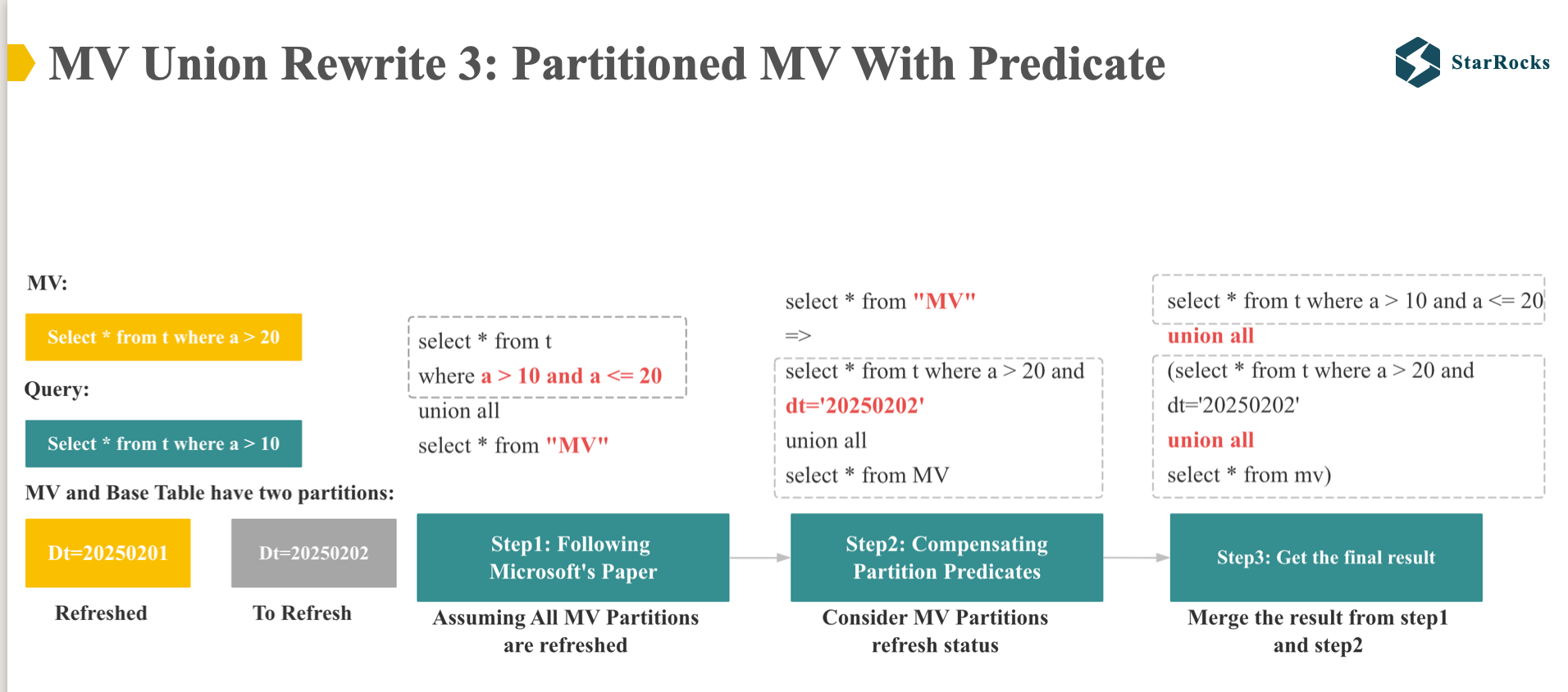
Finally, let’s consider the case of Partitioned MV With Predicate rewrite

Let’s illustrate this with an example. Imagine our base table is partitioned into ‘0201’ and ‘0202’. The Materialized View for partition ‘0201’ is up-to-date and refreshed, while the MV for ‘0202’ is stale and to refresh.

• The MV is defined as: SELECT * FROM t WHERE a > 20.
• Our query is: SELECT * FROM t WHERE a > 10.

1. We begin by assuming all MV partitions are refreshed, ignore the mv partition status for now. In this phase, we apply the rewriting techniques outlined in the Microsoft paper.

2. Then in the second step, we consider MV freshness and partition refresh status, add the partition compensation predicate to “MV scan” in the first step.

3. Finally, we merge the results of the first two steps to get the final result.

The Challenges Of CBO And StarRocks Solutions

The Challenges Of CBO

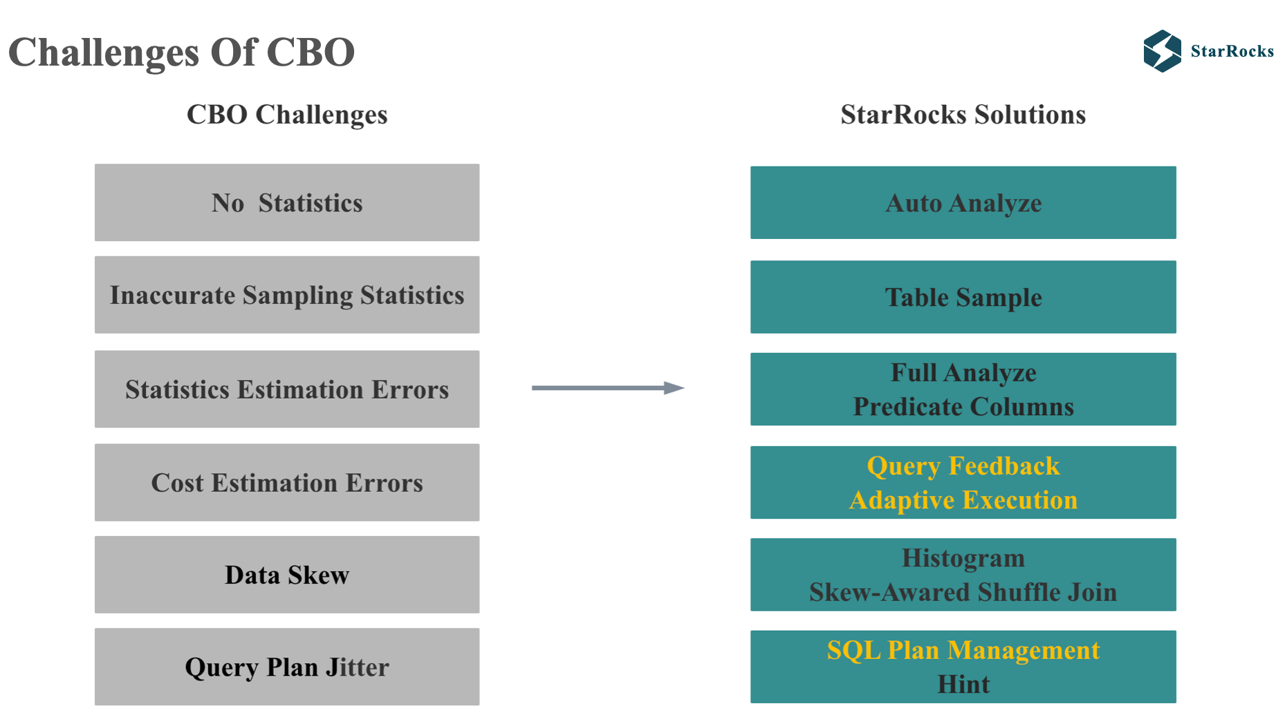
Over the past several years, we have continued to encounter many challenges in the cost estimation, which are also challenges that all CBO optimizers will encounter: For example:

• No statistical information
• Inaccurate collection of sampling statistical information
• Inaccurate estimation of sampling statistical information
• Even if the statistical information is accurate, the cost estimation will be wrong (because the basic assumptions of independence and irrelevance are not valid, or the errors of multi-level joins are amplified layer by layer)
• There are also common data skew problems in production environments
• There are also problems with production environment plan jitters exposed by some users in the past year, which will cause normal small queries to become large queries, leading to production environment accidents.

Today I will mainly introduce query feedback, adaptive execution and SQL plan management.

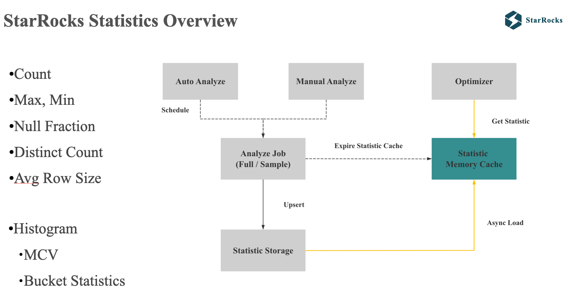
Before diving into these advanced features, let’s briefly review the basics of StarRocks Statistics.

First, StarRocks’ single-column statistics include basic count, max, min, Distinct, and also support Histogram.

StarRocks’ statistics support manual and automatic collection, and each collection supports both full and sampling methods.

To minimize query planning latency, statistics are cached in the Frontend memory, allowing the optimizer to efficiently retrieve column statistics directly from memory.

By default, StarRocks’ automatic collection employs a strategy of performing full ANALYZE on smaller tables and sample ANALYZE on larger tables.

The difficulty of collecting statistical information is to make a trade-off between resource consumption and accuracy, while also avoiding the statistical information collection task from affecting normal import and query.

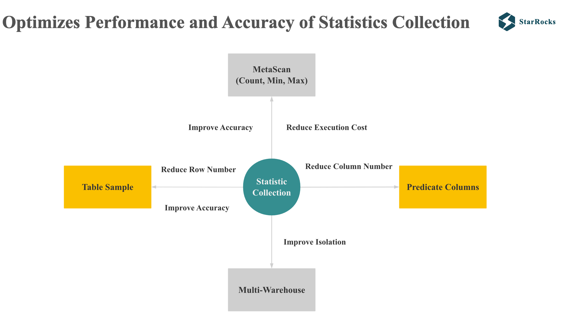
StarRocks optimizes the accuracy and performance of statistics collection in the following four aspects.

• The first point is meta scan. StarRocks uses meta scan to optimize the statistics of count, min, and max, reducing resource consumption.

• The second point is table sampling. When sampling, it will improve accuracy as much as possible while only scanning a small amount of data.

• StarRocks will reduce the cost of statistics collection by reducing both the number of collection rows and columns. The third point is predicate columns. Table sampling and predicate columns will be introduced soon.

• The last point is to reduce the impact of statistics collection on normal queries and ingestion. StarRocks currently supports executing statistics tasks in a separate warehouse, which ensures that the statistics collection job will not affect query and ingestion.

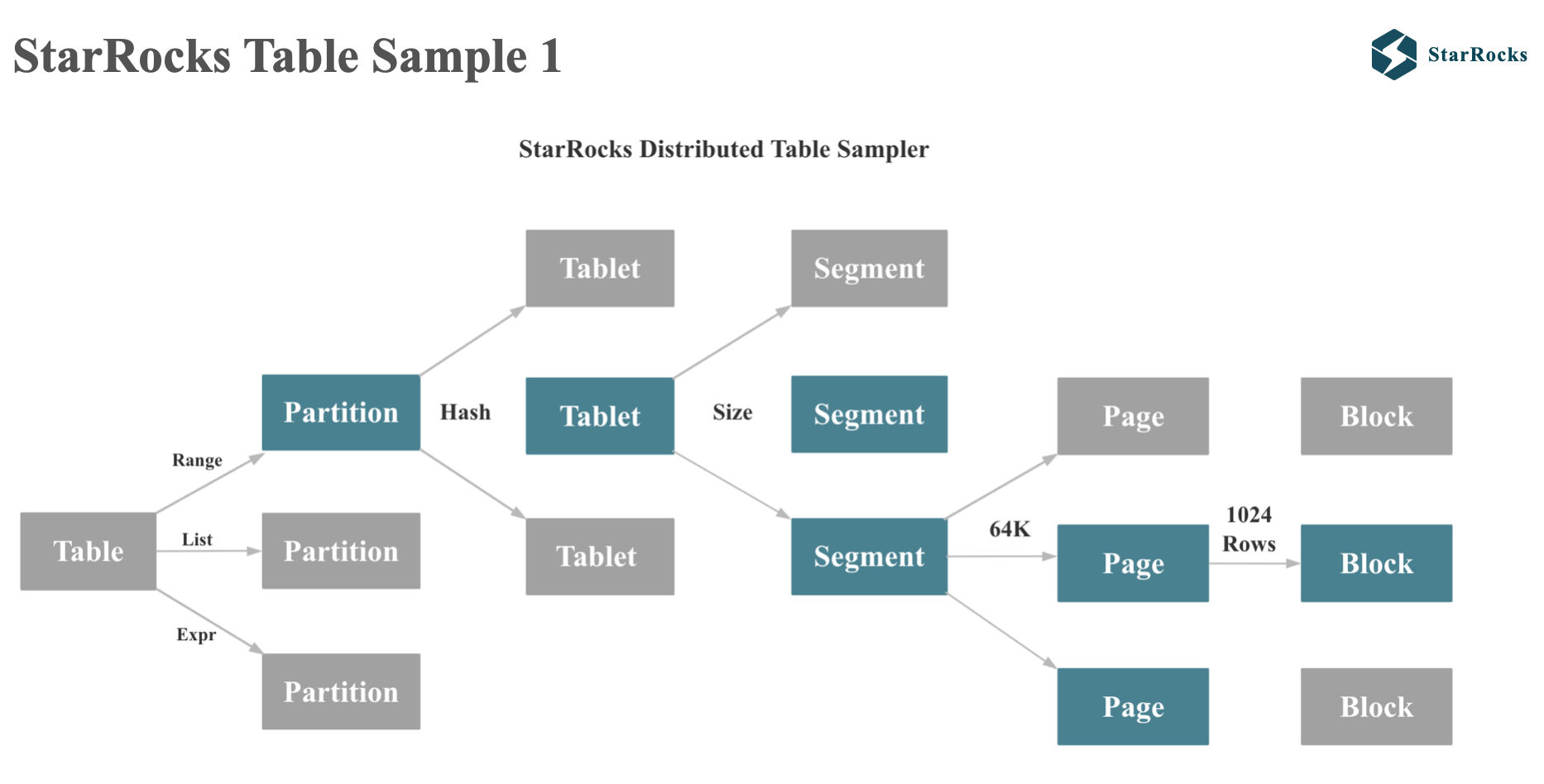
StarRocks’ table sampling will follow the actual physical distribution of table data.

As you can see from the diagram, StarRocks’ table will first be partitioned by range or list, and then followed by hash or random bucketing. Each tablet will be divided into multiple segments according to size. Each column of a segment will be divided into multiple pages according to 64kb each.

When StarRocks performs sampling statistics, it will read data from some tablets and some segments.

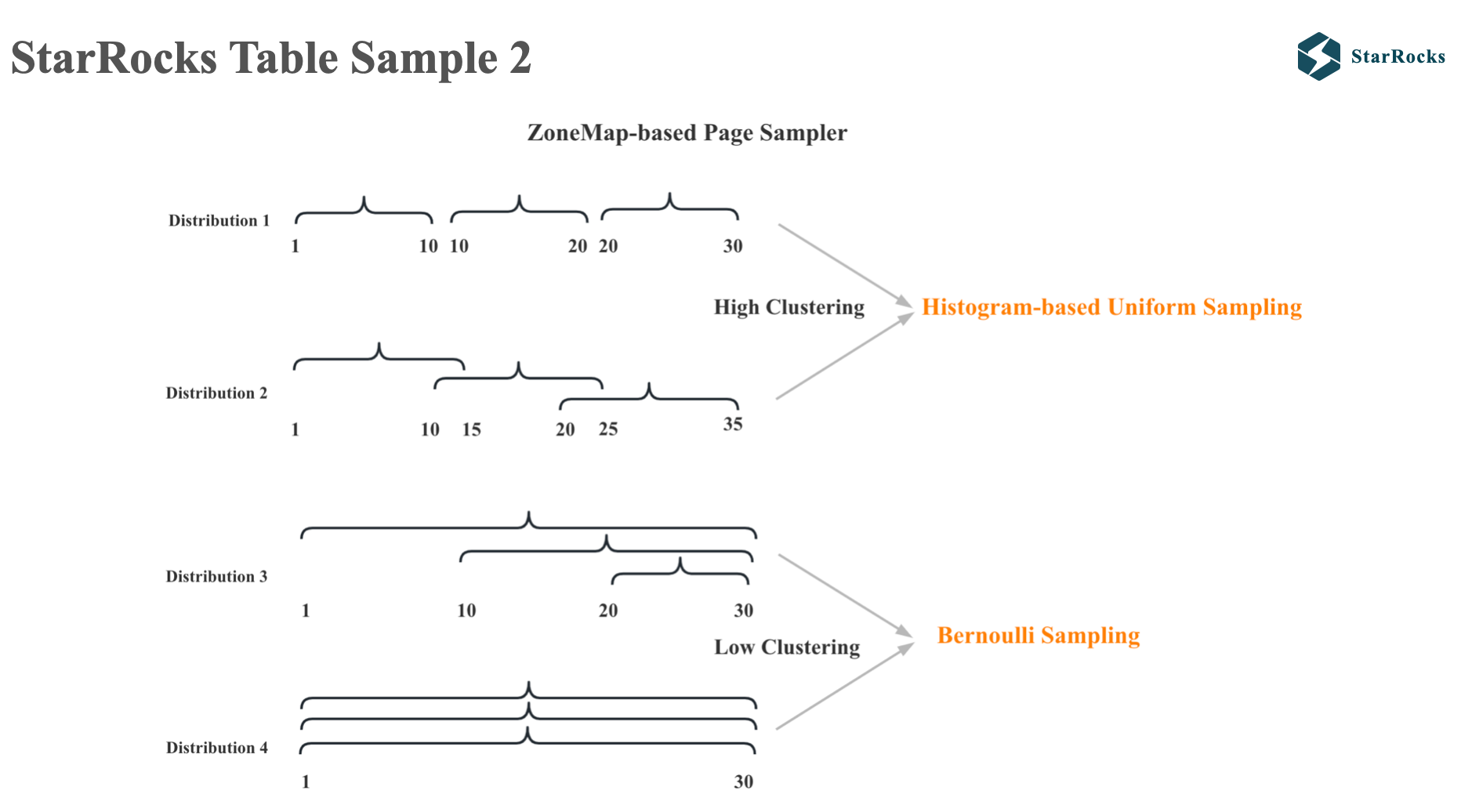
As for which pages of data to read in each segment, StarRocks will use different sampling algorithms according to different data distribution characteristics. StarRocks will first sort the pages according to the max and min values of each page’s zone map. If the data is found to be highly clustered, the histogram based uniform sampling algorithm will be used. If the data is found to be less clustered, the Bernoulli sampling algorithm will be used.

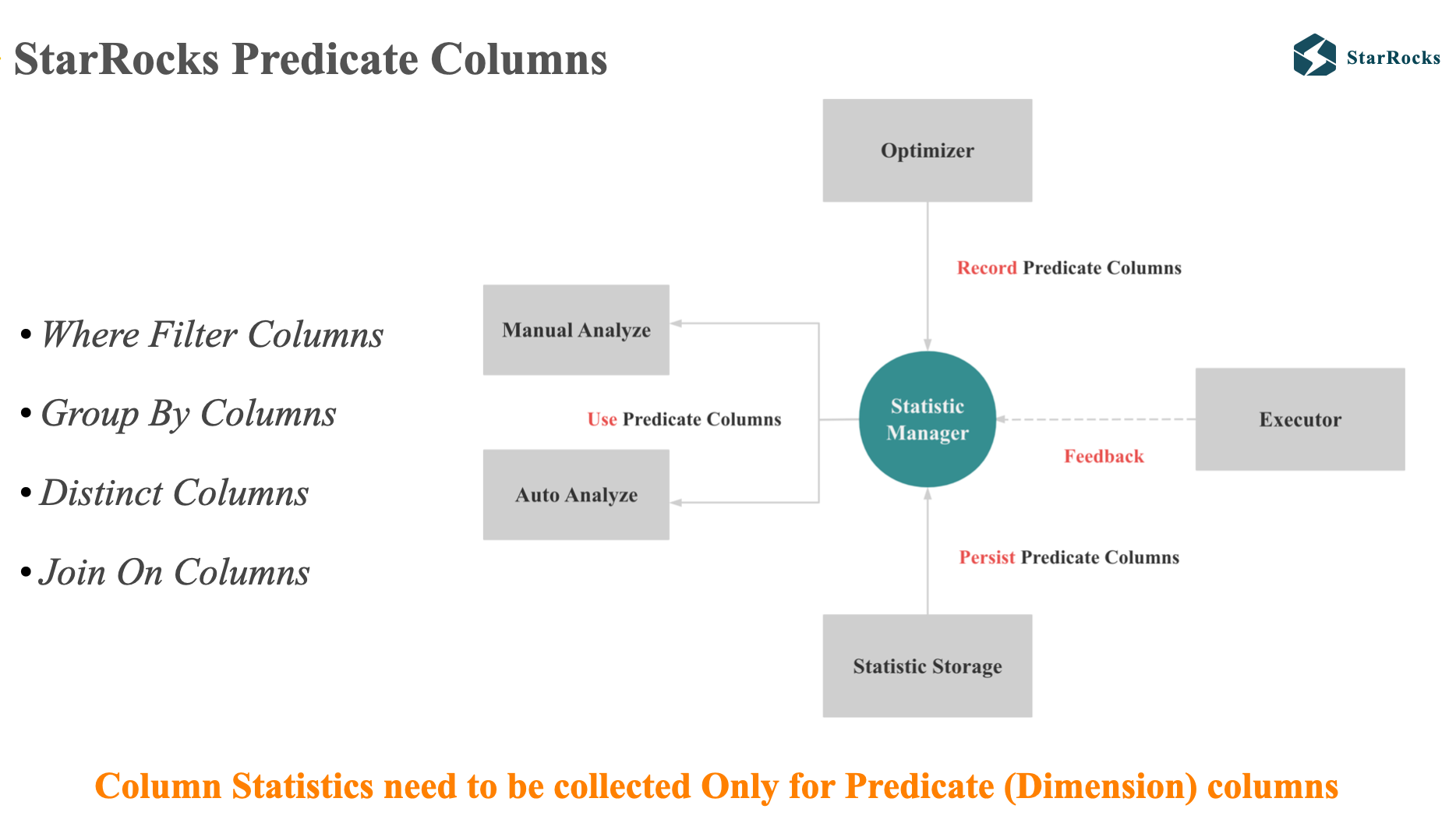
The core idea of the Predicate Columns mentioned before is very simple. We believe that when a table has hundreds or thousands of columns, only the statistical information of a few key columns will affect the quality of the final plan. In OLAP analysis, these columns are generally dimension columns, such as filter column, group by column, distinct column, and join on columns. So we only need to collect statistics for Predicate Columns

StarRocks Query Feedback

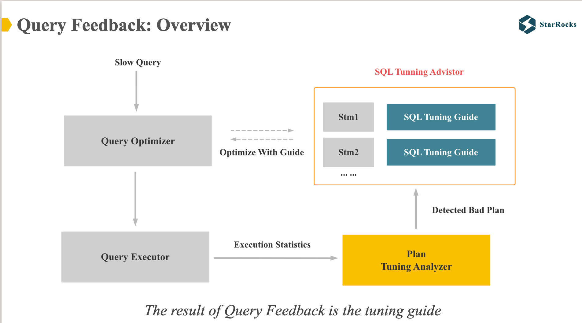
As mentioned earlier, query feedback is used to solve the problem of inaccurate cost estimation caused by any reason. The core idea is to use real runtime information to correct the bad query plan so that the optimizer can generate a better plan next time.

StarRocks’ query feedback does not update statistical information, but records the better tuning guide for each type query.

As shown in the diagram, Query Feedback has two core modules: plan tuning analyzer and sql tuning advisor.

Plan tuning analyzer checks whether there is a clear bad plan based on the real runtime information and execution plan of the query.If a clear bad plan is detected, it will be recorded.

When the optimizer generates the final plan, if it finds that the corresponding tuning guide is recorded in the sql tuning advisor, it will apply the better plan in the tuning guide.

Currently, the first version of query feedback can mainly optimize three types of cases:

• Optimize the left and right order of Join
• Optimize the distributed execution mode of Join (eg: broadcast -> shuffle)
• For cases where first-phase aggregation works well, disable streaming aggregation and aggregate more data in the first phase.

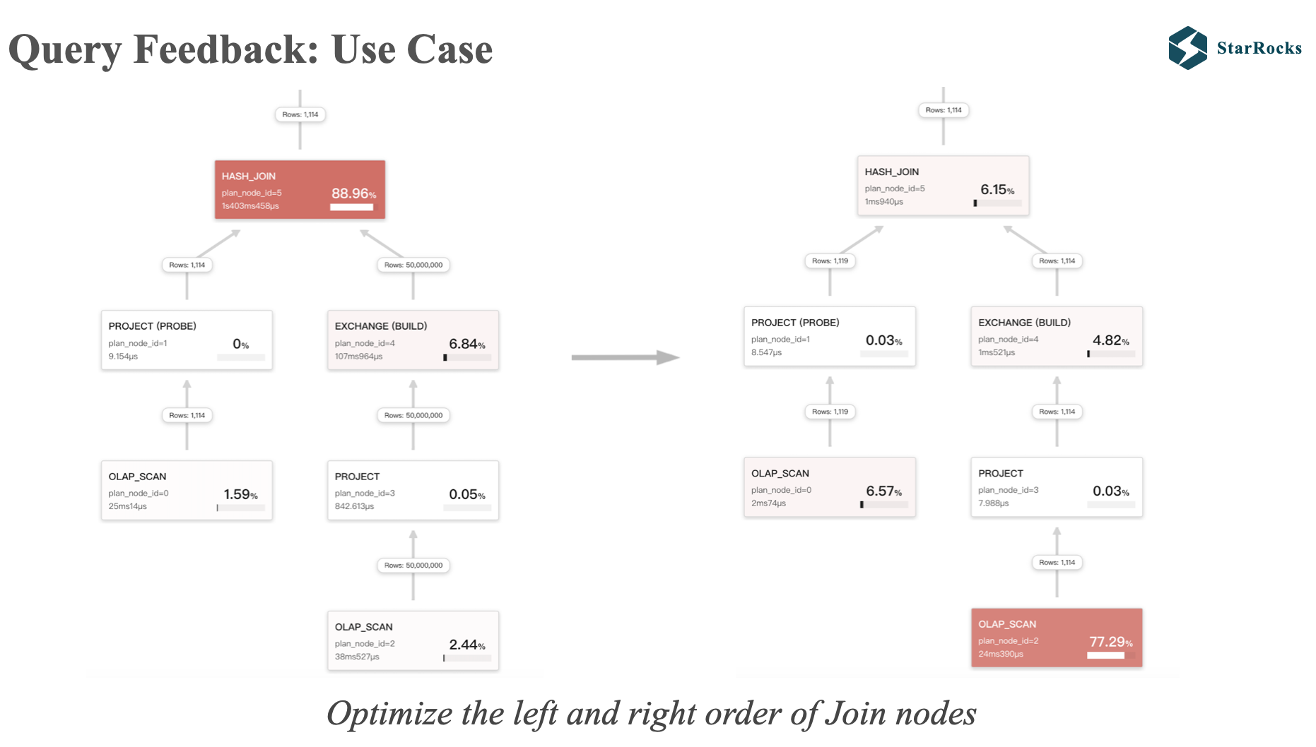
This is a use case of Query Feedback, which corrects the incorrect order of the left and right tables.

On the left query profile, there is a large table with 50,000,000 rows on the right, and a small table with 1,114 rows on the left. When the large table is used to build a hash table, the performance will be very poor.we should use the small table to build the hash table.

After applying feedback tuning, The join order become right.

At the same time, you can also find that in the right query profile, there are only 1,119 rows of data in the left table. This is because the runtime filter is effective and the data in the left table is filtered out. I will introduce the runtime filter later. You can see that the query time of the two different plans is an order of magnitude different.

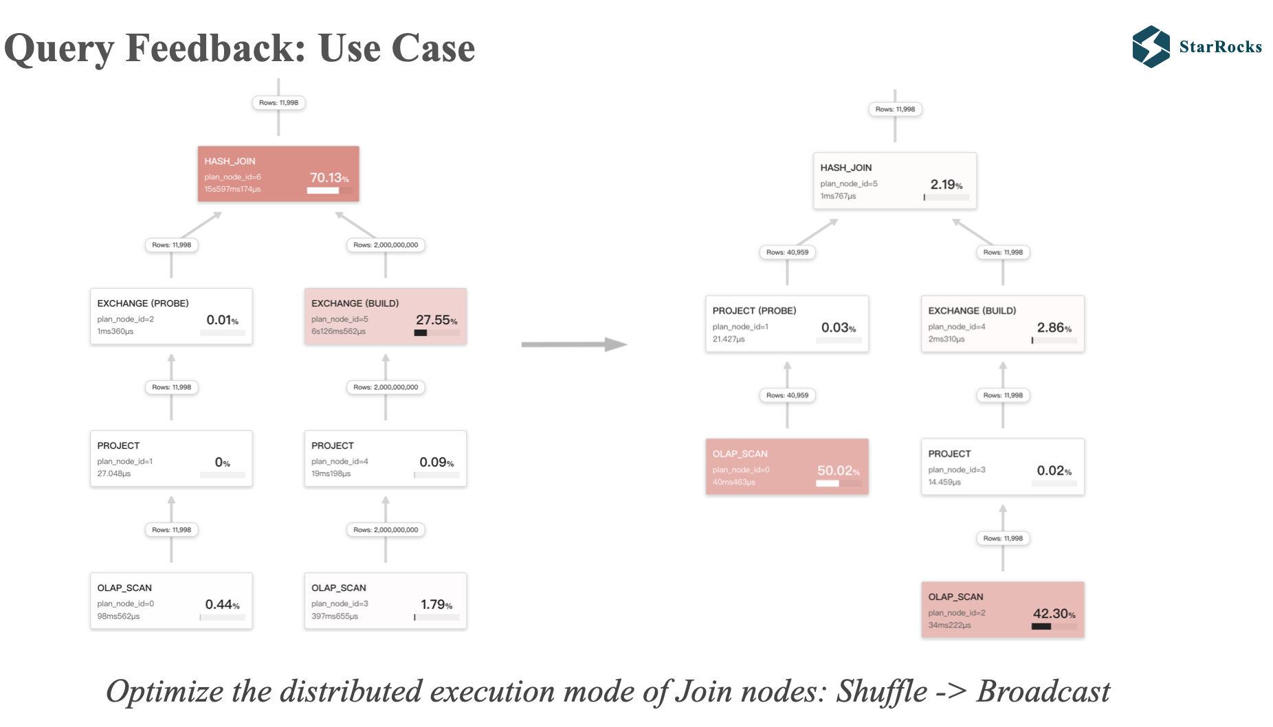
This is the second use case of query feedback, adjusting the incorrect shuffle join to broadcast join

As illustrated in the diagram, the left and right children of the left join are both exchanges, indicating shuffle join, but we found that the data in the left table only has 11,998 rows, and broadcast join is obviously a better execution strategy.

After applying feedback tuning, shuffle join is adjusted to broadcast join, and runtime filter is also effective. At the same time, you can also see that the query time of the two different plans is also orders of magnitude different.

StarRocks Adaptive Execution

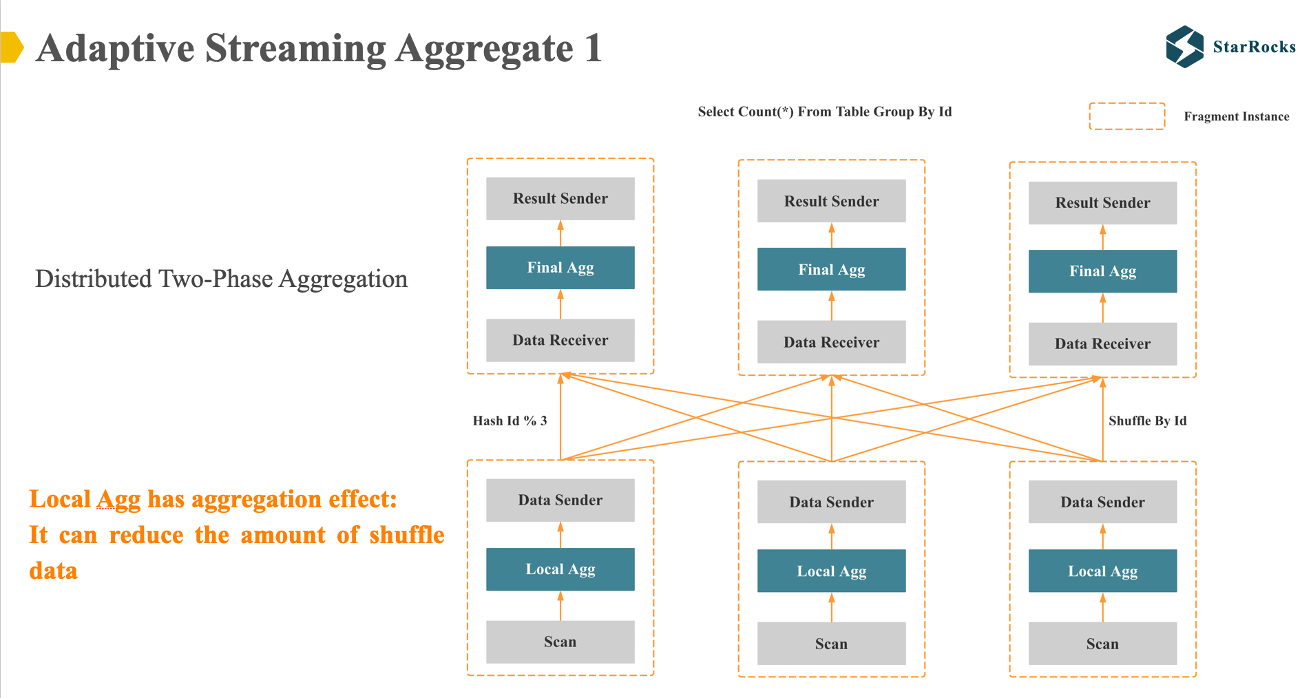
For a simple group by query: select count(*) from table group by id, if it is a non-colocate table, StarRocks will generate two distributed execution plans.

The first plan is a distributed two-phase execution: As illustrated in the diagram, in the first phase, StarRocks will first aggregate the data using a hash table according to the id column, and then send the data with the same id to the same node through hash shuffle. In the second phase, a final hash aggregation will be performed, and then the result will be returned to the client.

Why do we need to perform a local aggregation in the first phase? Because we expect to reduce the amount of data transmitted by the shuffle network through the first aggregation. Obviously, the assumption here is that the first local aggregation will have an aggregation effect, such as, the input rows is one million rows, after hash aggregate, the hash table size is only one thousand.

So, the two phase aggregation plan is generally suitable for medium and low cardinality group by columns.

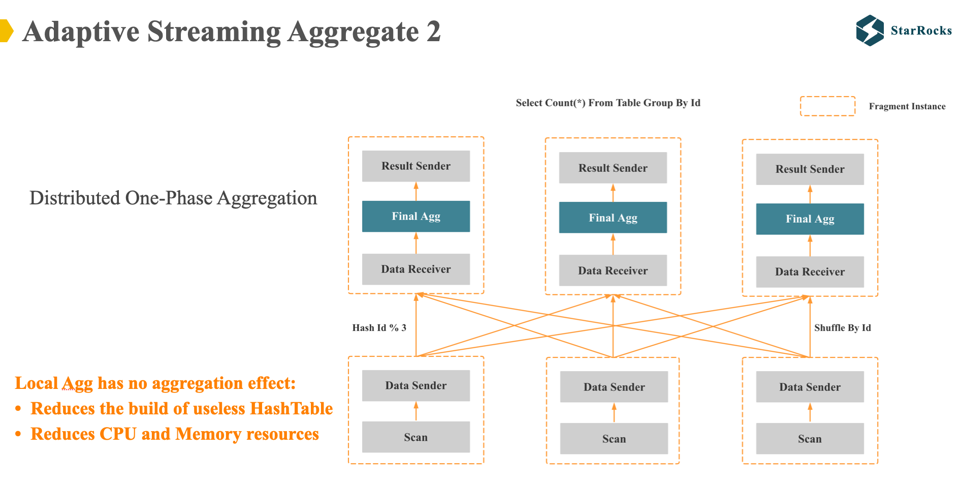
The second distributed execution plan of StarRocks group by is one-phase aggregation: that is, shuffle the data directly after scanning the data, and only do the final aggregation.

Obviously. One-phase aggregation is suitable for cases where local aggregation has no aggregation effect (such as, the input rows is one million rows, after hash aggregate, the hash table size is still one million.). So the one phase aggregation is suitable for high-cardinality group by columns.

In theory, as long as the optimizer can accurately estimate the cardinality of group by, we can directly select the correct one or two phase plan. However, for multi-column group by cardinality estimation, this is very challenging, because the multiple columns of group by are generally not independent and correlated.

Therefore, in Starrocks, we did not solve this problem in the optimizer direction, but hoped to solve this problem adaptively at the execution layer:

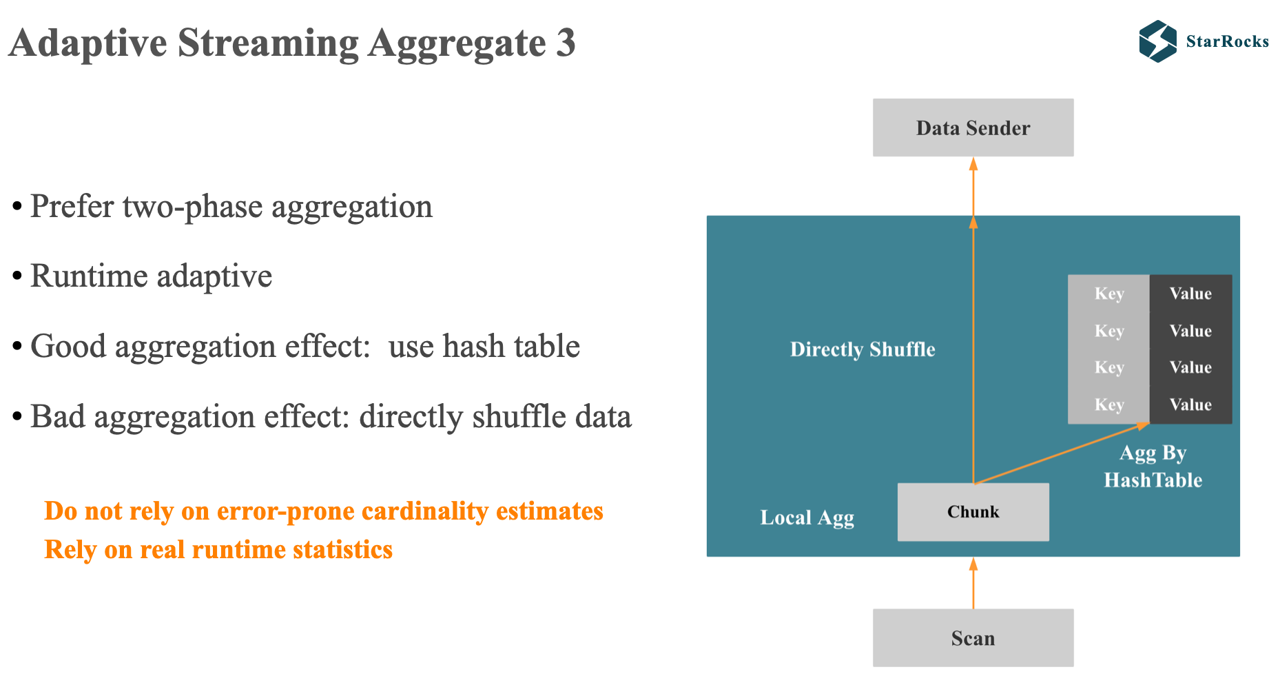
The starrocks optimizer will generate a distributed 2-phase aggregation plan by default. Then it will adaptively adjust aggregation strategies according to the actual aggregation effect obtained during execution.

As illustrated in the diagram, the principle of starrocks adaptive aggregation is as follows:

In local aggregation, for each batch of data, assuming 1 million rows, starrocks will first use the hash table to aggregate the data. When it is found that there is no aggregation effect, it will no longer add the data to the hash table, but directly shuffle to avoid meaningless hash aggregation.

This is the core idea of adaptive aggregation. The specific algorithm is relatively complex. In the past 5 years, we have optimized several versions, and we will not go into it in depth today. But if you are interested, we can discuss offline.

Next, let’s look at another case of adaptive execution: Adaptive Runtime Filters Selection. First, let’s quickly understand what runtime filter is. In some papers, runtime filter is also called Sideways information passing.

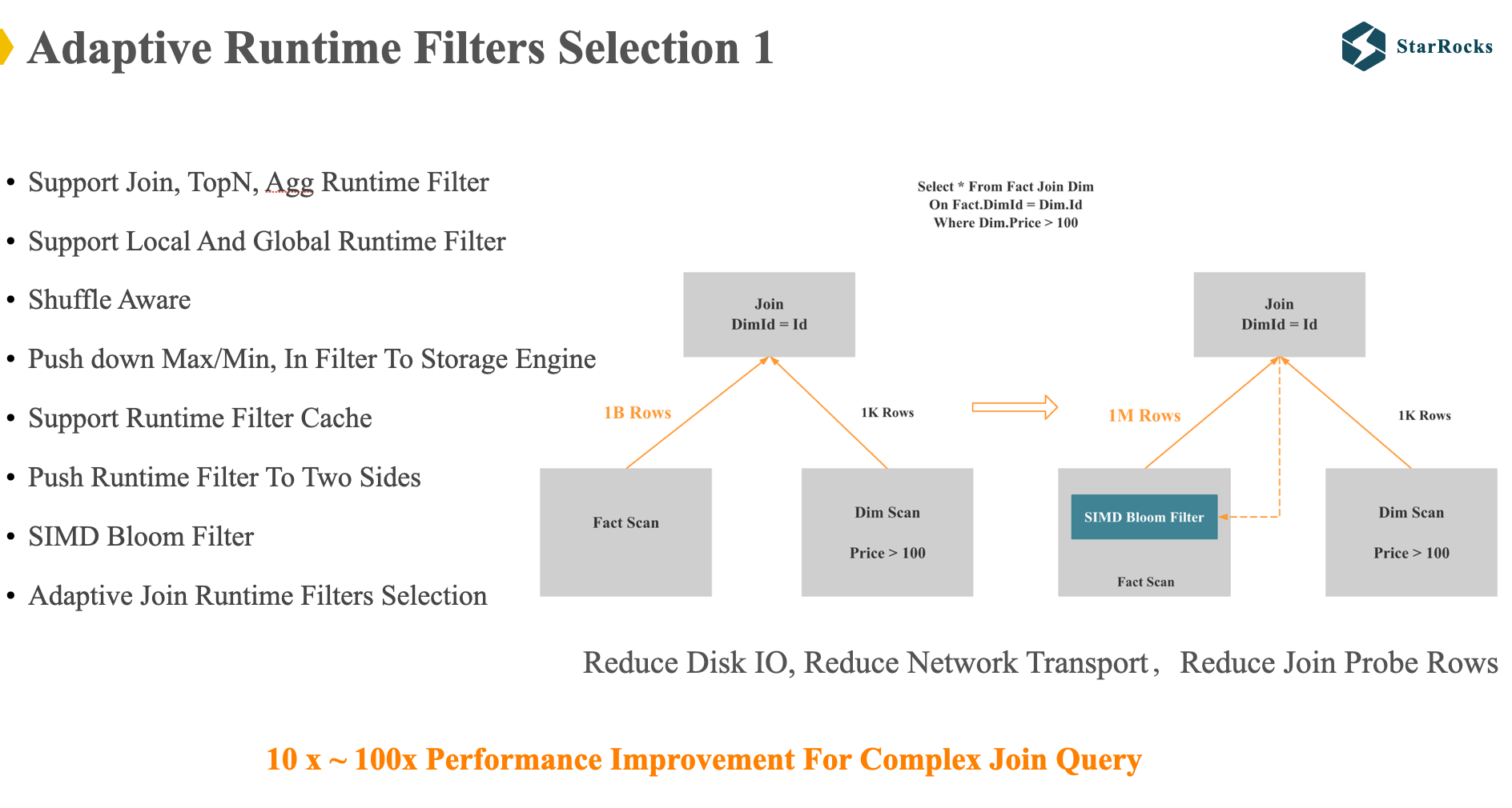
The figure is a simple schematic diagram of join runtime filter. After scanning the right table data, Starrocks will build a Runtime filter for the right table data and push it down to the left table. Runtime filter can filter the data in the left table before joining, reducing IO, network and CPU resources.

For complex SQL, runtime filter will have dozens of times performance improvement. In the past five years, Starrocks has been continuously improving runtime filter. Listed on the left are some features of the Starrocks runtime filter.

However, runtime filters may have negative optimization: when there are many join tables and many join on conditions, many runtime filters may be pushed down to the same scan node, which will lead to the following issues:

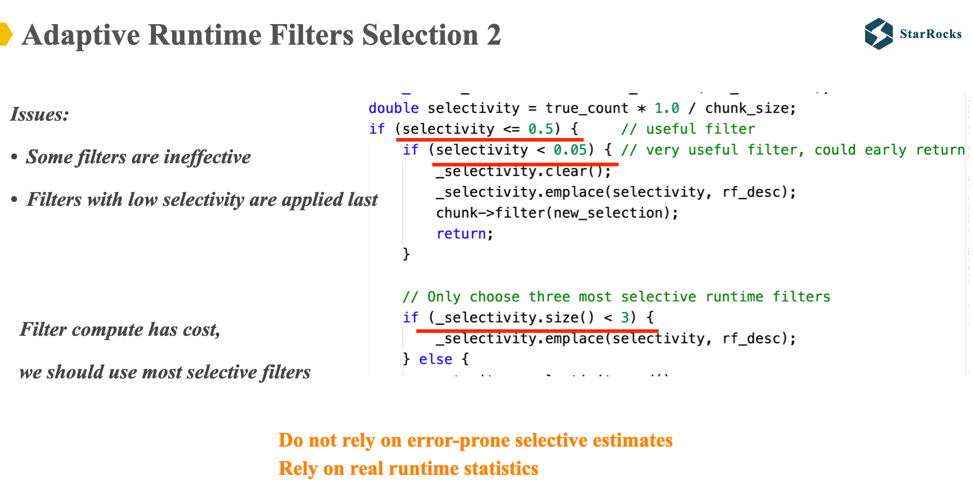
1. Some runtime filters are ineffective, wasting CPU resources
2. Filters with low selectivity are used last, and some filters with high selectivity are applied first, which also wastes CPU resources

Some databases may rely on the optimizer to estimate the selectivity of the runtime filter, but Starrocks chooses to use Adaptive execution to solve this problem.

As illustrated in the diagram, Starrocks computes the actual selectivity of each runtime filter after a certain number of rows of data, and then adaptively adjusts the application of the runtime filter. Here are some basic adjustment principles:

1. Only select filters with lower selectivity
2. Only select 3 filters at most
3. If the selectivity of a filter is particularly low, only keep one filter

SQL Plan Management

Finally, let’s introduce SQL Plan Management. We are currently developing this feature and will release the first version soon.

We decided to develop this feature because over the past year or so, some users’ online small queries became large queries due to plan jitter, which led to production accidents.

Our aim with SQL Plan Management is to address two critical challenges:

1 Preventing performance regressions after upgrades: We want to guarantee that query performance remains stable and predictable, eliminating significant slowdowns caused by plan changes following system upgrades.

2 Maintaining stable performance for critical online workloads: We seek to ensure that the query plans for essential, continuously running business applications remain consistently efficient, avoiding performance degradation over time.

SQL Plan Management is divided into two parts in principle:

1. How to generate and save the baseline plan
2. How to apply the baseline plan

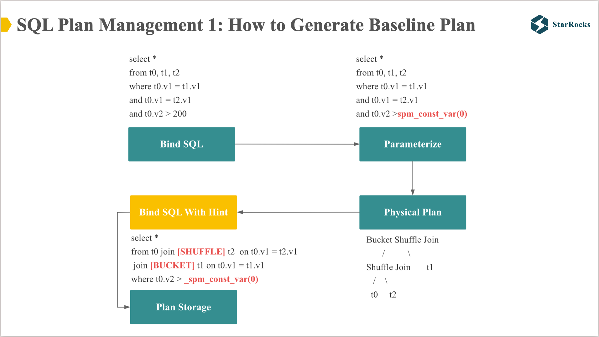
How to generate the Baseline Plan is divided into 3 steps:

1. Parameterization of constants: replace the SQL constants with special SPMFunctions
2. Generate plan: generate a distributed physical plan based on the parameterized plan，you could see which is shuffle join and bucket shuffle join. the bucket shuffle join means only shuffle one table data to another table, another table data remain unchanged.
3. Generate baseline SQL: convert the physical plan into SQL with hints. In starrocks, if a join has a join hint, starrocks won’t do join reorder, so the shuffle and bucket hints almost determine the two key points of this SQL plan: join order and join distributed execution strategy.

why starrocks save the bind sql with hint, not the physical plan, which because:

1. save the storage space, the physical plan may be large
2. sql with hint is easier to Validate

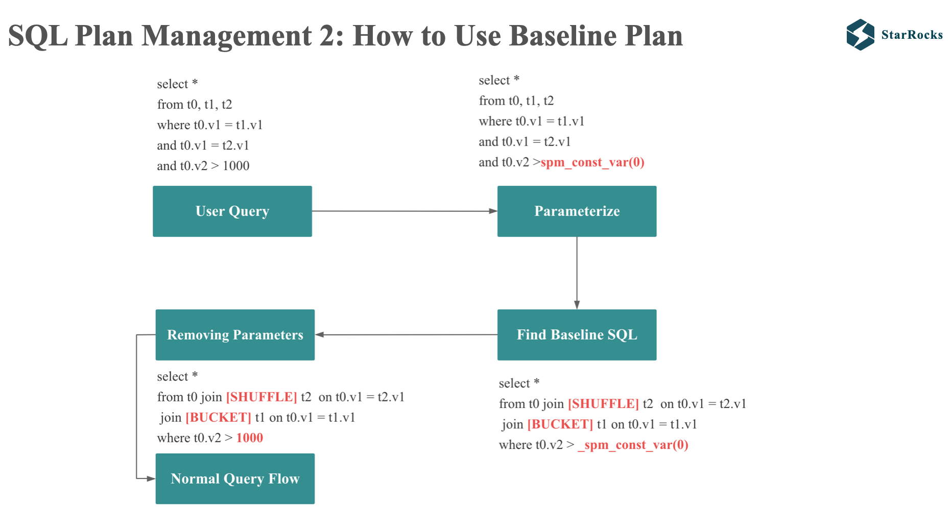
Using baseline plan is divided into 4 steps:

1. Parameterization of constants: replace the query constants with special SPMFunctions
2. Get baseline SQL: calculate the digest of the parameter SQL, and find the corresponding baseline SQL in plan storage according to the digest
3. Replace the SPMFunctions in the baseline SQL with the constants of the input SQL
4. Then process the SQL with hint according to the normal query process

FAQ

StarRocks Join Reorder Algorithm

StarRocks optimizer implements multiple Join Reorder algorithms, using different algorithms according to different Join numbers:

• When the number of Joins is less than or equal to 4, use Join associative law + Join commutative law
• When the number of Joins is less than or equal to 10, use left-deep tree + dynamic programming algorithm + greedy algorithm
• When the number of Joins is less than or equal to 16, use left-deep tree + greedy algorithm
• When the number of Joins is less than or equal to 50, use left-deep tree
• When the number of Joins is greater than 50, do not perform Join Reorder

How to optimize the combinatorial explosion problem of Join Reorder and distributed strategies

1. Limit the number of Join Reorder results

   1. Left-deep tree and dynamic programming algorithms will only produce one Join Reorder result
   2. Greedy algorithm will only take the top K Join Reorder results

2. When exploring the search space, pruning will be performed based on the lower bound and upper bound

Do Query Feedback and Plan Management support parameterization?

The first version does not support this feature yet, but we will support it soon this year. The idea is to divide the parameter range into ranges, so that scenario parameters in different ranges correspond to different tuning guides and different baseline plans.

Lessons From StarRocks Query Optimizer

1. Errors in optimizer cost estimation are unavoidable, and the executor needs to be able to make autonomous decisions and provide timely feedback. so I think the Adaptive Execution and Query Feedback are necessary for a cost-based optimizer
2. In engineering, the optimizer testing system is as important as the optimizer itself. The optimizer requires correctness testing, performance testing, plan quality testing, etc.I believe that our open-source database ecosystem would benefit from an open-source testing system for optimizers and queries, along with a publicly available test dataset. This could significantly accelerate the transition of database optimizers from demonstration to maturity.
3. Null and Nullable is Interesting and Annoying
   • For Performance, we need to special handle Null and nullable, Especially if your query executor is a vectorized executor
   • For Correctness, we need to take care of Null and nullable in Optimizer and Executor
4. Integrated optimizer could be more powerful than Standalone optimizer
   • Because the integrated optimizer can more easily obtain more context, it is easier to do more optimizations, such as global dict optimization, query feedback, etc.

Summary

Due to time constraints, this sharing mainly shared three representative optimizations of the StarRocks query optimizer and solutions to cost estimation challenges. If you are interested in other parts of the StarRocks query optimizer, you are welcome to communicate.